NetPyNE Tutorial
This tutorial provides an overview of how to use the NetPyNE Python package to create a simple simulation of a network of neurons.
Downloading and installation instructions for NetPyNE can be found here: Installation
A good understanding of Python nested dictionaries and lists is recommended, since they are are used to specify the parameters. There are many good online Python courses available, e.g. from CodeAcademy or Google.
See also
For a comprehensive description of all the features available in NetPyNE see User Documentation.
Tutorial 1: Quick and easy example
To start in an encouraging way, we will implement the simplest example possible consisting of just three lines! This will create a simple network (200 randomly connected cells), run a one-second simulation, and plot the network spiking raster plot and the voltage trace of a cell.
You will need to download the HHTut.py example parameter file (download here - right click and “Save as” to same folder you are working in).
The code looks like this (available here tut1.py):
import HHTut
from netpyne import sim
sim.createSimulateAnalyze(netParams = HHTut.netParams, simConfig = HHTut.simConfig)
The first line imports the HHTut module with the network and simulation parameters.
The second line imports the sim module from the netpyne package. The sim module provides functions to easily create and simulate networks based on these parameters.
The third line calls the createSimulateAnalyze function, which runs a standard sequence of commands to create and simulate the network, and save and plot data. It requires the following two arguments:
netParams- an object of class NetParams to store network parameters (e.g. cell properties, populations, connectivity)simConfig- an object of class SimConfig to store simulation options (e.g. duration, dt, recording and plotting options, etc.)
In this case we are using a set of predefined parameters specified in the HHTut module (Hodgkin-Huxley network example). The HHTut module contains the two required objects: netParams and simConfig.
To run the model just execute the tut1.py script. One way to do this is to run this shell command:
python tut1.py
If you successfully installed MPI (e.g. OpenMPI) and NEURON with MPI support, you can simulate the model in parallel using multiple cores/processors by typing:
mpiexec -n 4 nrniv -python -mpi tut1.py
where you would replace the 4 with the number of cores you want to use.
If you want to avoid typing that long line every time, you can download this simple shell script (runsim) and just type:
./runsim 4 tut1.py
Note
To use the script make sure you change its permissions so it is executable (e.g. chmod +x runsim).
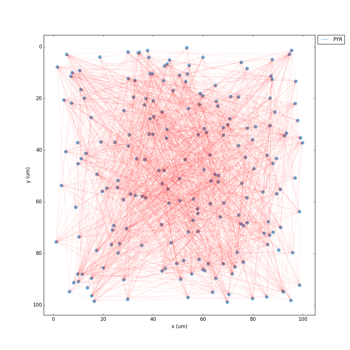
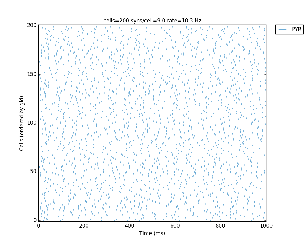
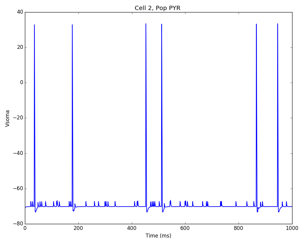
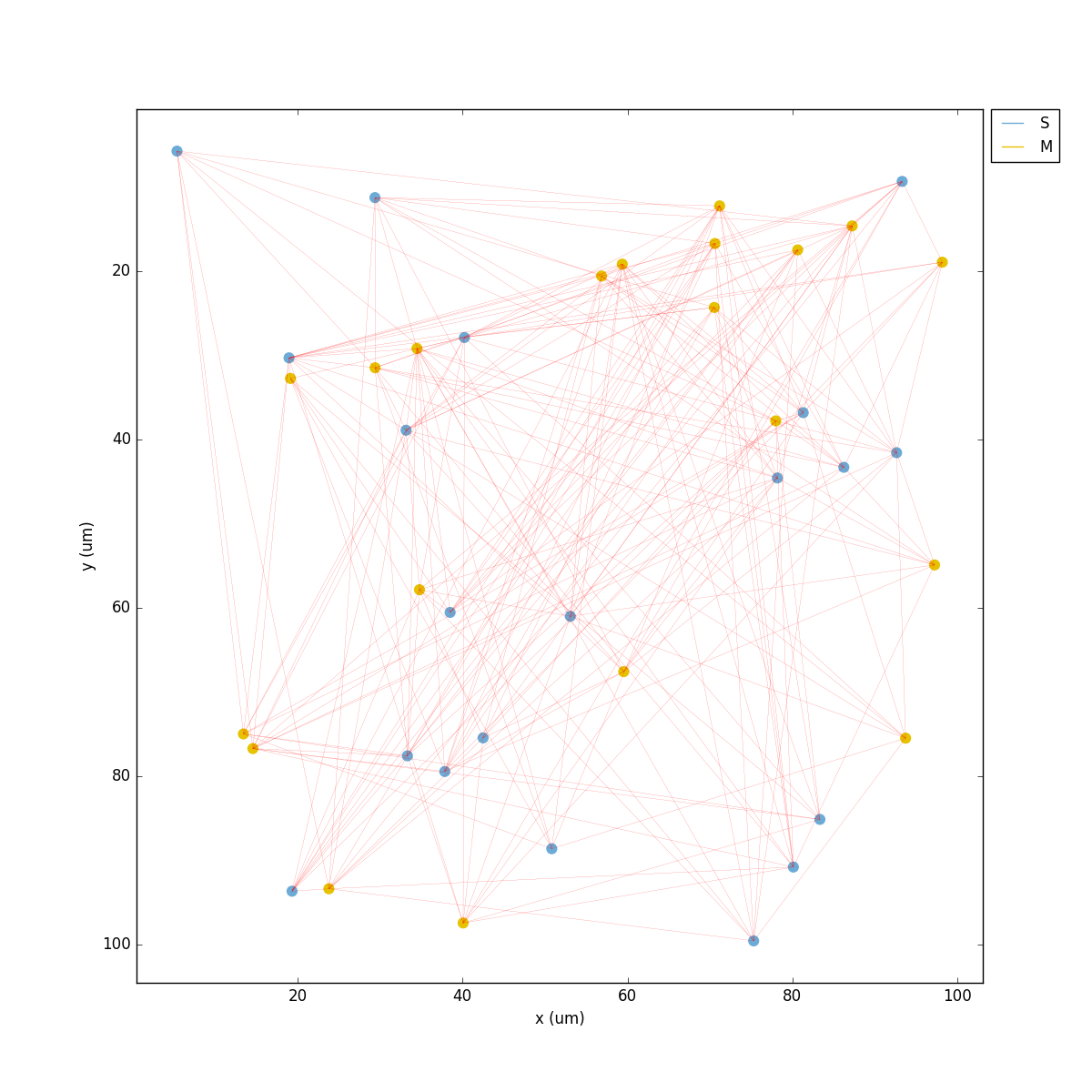
Whatever method you use, you should get a 2D representation of the cells and connections in the network, a raster plot (spikes as cell versus time) and the voltage trace of a single cell:
Congratulations! You have created and simulated a biological neuronal network in NEURON!
Note
In some systems the figures that appear may be empty. This can be fixed by adding this line to the end of your tut1.py: import pylab; pylab.show() . In any case, the raster plot and the voltage trace figures will be correctly saved to disk as HHTut_raster.png and HHTut_traces.png.
In the remainder of this tutorial we will see how to easily specify your own parameters to create custom networks and simulations. For simplicity, the network parameters, simulation options and calls to functions (necessary to create the network, simulate it and plot the results) will all be included in a single file. For larger models it is recommended to keep model specification parameters and function calls in separate files (see examples here.)
We begin with an overview of the Python objects where you will define all your network parameters.
Tutorial 2: Network parameters
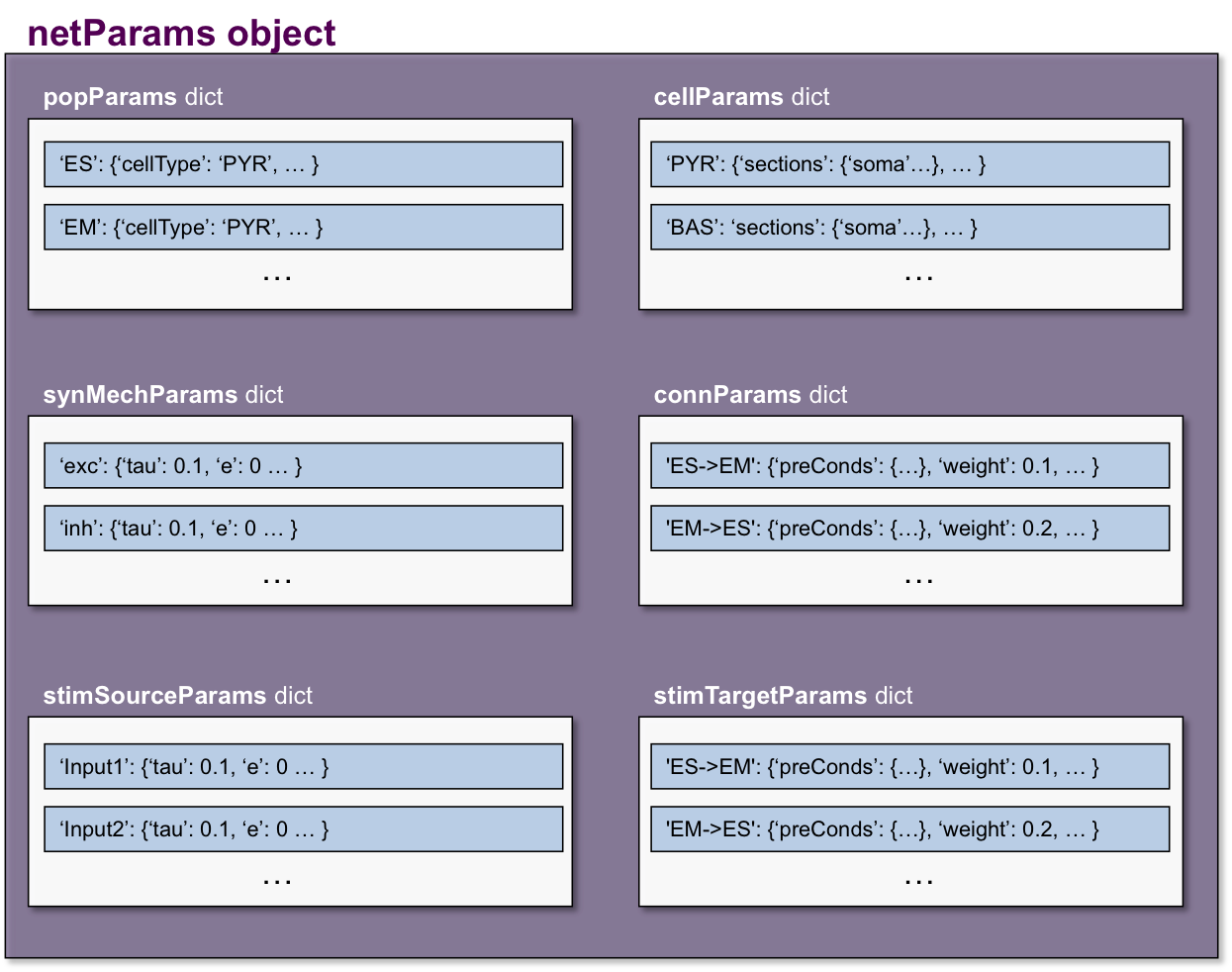
The netParams object includes all the information necessary to define your network. It is composed of the following 8 ordered dictionaries:
cellParams- cell types and their associated parameters (e.g. cell geometry)popParams- populations in the network and their parameterssynMechParams- synaptic mechanisms and their parametersconnParams- network connectivity rules and their associated parameters.subConnParams- network subcellular connectivity rules and their associated parameters.stimSourceParams- stimulation sources parameters.stimTargetParams- mapping between stimulation sources and target cells.rxdParams- reaction-diffusion (RxD) components and their parameters.
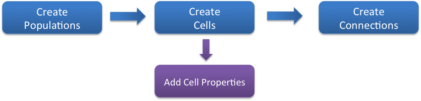
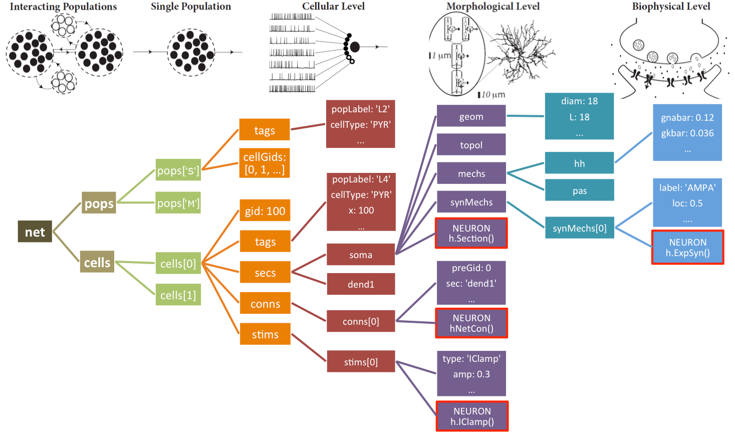
The netParams organization is consistent with the standard sequence of events that the package executes internally:
creates a
Networkobject and adds inside a set ofPopulationandCellobjects based onpopParamssets the cell properties based on
cellParamscreates a set of connections based on
connParamsandsubConnParams(checking which presynpatic and postsynaptic cells match the conn rule conditions), and using the synaptic parameters insynMechParams.add stimulation to the cells based on
stimSourceParamsandstimTargetParams.
The image below illustrates this process:
We will now create a new model file (call it tut2.py) where we will specify from scratch all the network parameters. To create the structures that will hold the network parameters add the following code:
from netpyne import specs, sim

# Network parameters
netParams = specs.NetParams()  # object of class NetParams to store the network parameters
Cell types
First, we need to define the properties of each cell type, by adding items to the cellParams dictionary. Each cellParams item includes a key (the cell type) and a value consisting of a dictionary with the following field:
secs- dictionary containing the properties of sections, e.g. geometry, mechanisms
In our example we create a cell type we’ll call PYR, which we will use in both our populations. We specify that we want them to have a section labeled soma with a certain geometry and a Hodgkin-Huxley mechanism (hh):
PYRcell = {'secs': {}}
PYRcell['secs']['soma'] = {'geom': {}, 'mechs': {}}
PYRcell['secs']['soma']['geom'] = {'diam': 18.8, 'L': 18.8, 'Ra': 123.0}                           # soma geometry
PYRcell['secs']['soma']['mechs']['hh'] = {'gnabar': 0.12, 'gkbar': 0.036, 'gl': 0.003, 'el': -70}  # soma hh mechanism
netParams.cellParams['PYR'] = PYRcell
Take a moment to examine the nested dictionary structure used to define the cell type. Notice the use of empty dictionaries ({}) and intermediate dictionaries (e.g. PYRcell) to facilitate filling in the parameters. There are other equivalent methods to add this rule, such as:
netParams.cellParams['PYR'] = {
        'secs': {'soma':
                {'geom': {'diam': 18.8, 'L': 18.8, 'Ra': 123.0},
                'mechs': {'hh': {'gnabar': 0.12, 'gkbar': 0.036, 'gl': 0.003, 'el': -70}}}}})
Populations
Now we need to create some populations for our network, by adding items to the popParams dictionary in netParams. Each popParams item includes a key (population label) and a value consisting of a dictionary with the following population parameters (see Population parameters for more details):
cellType- an attribute/tag assigned to cells in this population, can later be used to set certain cell properties to cells with this tag.numCells- number of cells in this population (can also specify using cell density)cellModel- an attribute or tag that will be assigned to cells in this population, can later be used to set specific cell model implementation for cells with this tag. e.g. ‘HH’ (standard Hodkgin-Huxley type cell model) or ‘Izhi2007b’ (Izhikevich 2007 point neuron model). Cell models can be defined by the user or imported.
We will start by creating two populations labeled S (sensory) and M (motor), with 20 cells each, of type PYR (pyramidal), and using HH cell model (standard compartmental Hodgkin-Huxley type cell).
## Population parameters
netParams.popParams['S'] = {'cellType': 'PYR', 'numCells': 20}
netParams.popParams['M'] = {'cellType': 'PYR', 'numCells': 20}
During execution, this will tell NetPyNE to create 40 Cell objects, each of which will include the attributes or tags of its population, i.e. ‘cellType’: ‘PYR’, etc. These tags can later be used to define the properties of the cells, or connectivity rules.
To get a better intuition of the data structure, you can print(netParams.popParams) to see all the populations parameters, or print print(netParams.popParams['M']) to see the parameters of population ‘M’.
Synaptic mechanisms parameters
Next we need to define the parameters of at least one synaptic mechanism, by adding items to the synMechParams dictionary. Each synMechParams items includes a key (synMech label, used to reference it in the connectivity rules), and a value consisting of a dictionary with the following fields:
mod- the NMODL mechanism (e.g. ‘ExpSyn’)mechanism parameters (e.g.
tauore) - these will depend on the specific NMODL mechanism.
Synaptic mechanisms will be added to cells as required during the connection phase. Each connectivity rule will specify which synaptic mechanism parameters to use by referencing the appropiate label. In our network we will define the parameters of a simple excitatory synaptic mechanism labeled exc, implemented using the Exp2Syn model, with rise time (tau1) of 0.1 ms, decay time (tau2) of 5 ms, and equilibrium potential (e) of 0 mV:
## Synaptic mechanism parameters
netParams.synMechParams['exc'] = {'mod': 'Exp2Syn', 'tau1': 0.1, 'tau2': 5.0, 'e': 0}  # excitatory synaptic mechanism
Stimulation
Let’s now add a some background stimulation to the cells using NetStim (NEURON’s artificial spike generator). We will create a source of stimulation labeled bkg and we will specify we want a firing rate of 100 Hz and with a noise level of 0.5:
# Stimulation parameters
netParams.stimSourceParams['bkg'] = {'type': 'NetStim', 'rate': 10, 'noise': 0.5}
Next we will specify what cells will be targeted by this stimulation. In this case we want all pyramidal cells so we set the conditions to {'cellType': 'PYR'}. Finally we want the NetStims to be connected with a weight of 0.01, a delay of 5 ms, and to target the exc synaptic mechanism:
netParams.stimTargetParams['bkg->PYR'] = {'source': 'bkg', 'conds': {'cellType': 'PYR'}, 'weight': 0.01, 'delay': 5, 'synMech': 'exc'}
Connectivity rules
Finally, we need to specify how to connect the cells, by adding items (connectivity rules) to the connParams dictionary. Each connParams item includes a key (conn rule label), and a values consisting of a dictionary with the following fields:
preConds- specifies the conditions of the presynaptic cellspostConds- specifies the conditions of the postsynaptic cellsweight- synaptic strength of the connectionsdelay- delay (in ms) for the presynaptic spike to reach the postsynaptic neuronsynMech- synpatic mechanism parameters to useprobabilityorconvergenceordivergence- optional parameter to specify the probability of connection (0 to 1), convergence (number of presyn cells per postsyn cell), or divergence (number of postsyn cells per presyn cell), respectively. If omitted, all-to-all connectivity is implemented.
We will add a rule to randomly connect the sensory to the motor population with a 50% probability:
## Cell connectivity rules
netParams.connParams['S->M'] = { #  S -> M label
        'preConds': {'pop': 'S'},   # conditions of presyn cells
        'postConds': {'pop': 'M'},  # conditions of postsyn cells
        'probability': 0.5,         # probability of connection
        'weight': 0.01,             # synaptic weight
        'delay': 5,                 # transmission delay (ms)
        'synMech': 'exc'}           # synaptic mechanism
Simulation configuration options
Above we defined all the parameters related to the network model. Here we will specify the parameters or configuration of the simulation itself (e.g. duration), which is independent of the network.
The simConfig object can be used to customize options related to the simulation duration, timestep, recording of cell variables, saving data to disk, graph plotting, and others. All options have defaults values so it is not mandatory to specify any of them.
Below we include the options required to run a simulation of 1 second, with integration step of 0.025 ms, record the soma voltage at 0.1 ms intervals, save data (params, network and simulation output) to a pickle file called model_output, plot a network raster, plot the voltage trace of cell with gid 1, and plot a 2D representation of the network:
# Simulation options
simConfig = specs.SimConfig()       # object of class SimConfig to store simulation configuration

simConfig.duration = 1*1e3          # Duration of the simulation, in ms
simConfig.dt = 0.025                # Internal integration timestep to use
simConfig.verbose = False           # Show detailed messages
simConfig.recordTraces = {'V_soma':{'sec':'soma','loc':0.5,'var':'v'}}  # Dict with traces to record
simConfig.recordStep = 0.1          # Step size in ms to save data (e.g. V traces, LFP, etc)
simConfig.filename = 'tut2'         # Set file output name
simConfig.savePickle = False        # Save params, network and sim output to pickle file

simConfig.analysis['plotRaster'] = {'saveFig': True}                  # Plot a raster
simConfig.analysis['plotTraces'] = {'include': [1], 'saveFig': True}  # Plot recorded traces for this list of cells
simConfig.analysis['plot2Dnet'] = {'saveFig': True}                   # plot 2D cell positions and connections
The complete list of simulation configuration options is available here: Simulation configuration.
Network creation and simulation
Now that we have defined all the network parameters and simulation options, we are ready to actually create the network and run the simulation. To do this we use the createSimulateAnalyze function from the sim module, and pass as arguments the netParams and simConfig dicts we have just created:
sim.createSimulateAnalyze(netParams, simConfig)
Note that as before we need to make sure we have imported the sim module from the netpyne package.
The full tutorial code for this example is available here: tut2.py
To run the model we can use any of the methods previously described in Tutorial 1: Quick and easy example:
If mpi not installed:
python tut2.py
If mpi working:
mpiexec -n 4 nrniv -python -mpi tut2.py
If mpi working and have runsim shell script:
./runsim 4 tut2.py
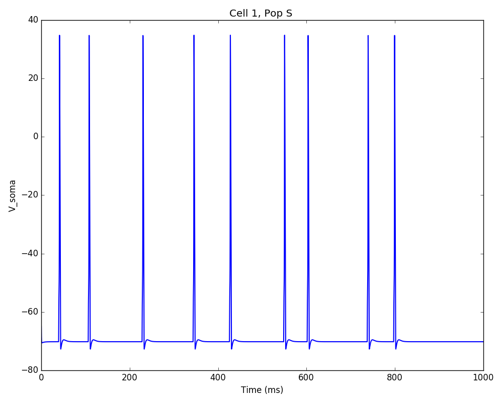
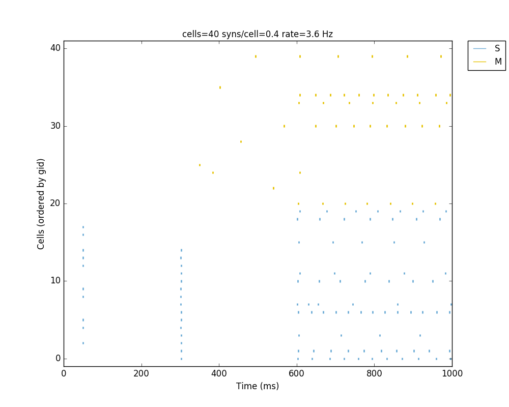
You should get the raster plot and voltage trace figures shown below. Notice how the M population firing rate is higher than that of the S population. This makes sense since they both receive the same background inputs, but S cells connect randomly to M cells thus increasing the M firing rate.

Feel free to explore the effect of changing any of the model parameters, e.g. number of cells, background or S->M weights, cell geometry or biophysical properties, etc.
Tutorial 3: Adding a compartment (dendrite) to cells
Here we extend the pyramidal cell type by adding a dendritic section with a passive mechanism. Note that for the dend section we included the topol dict defining how it connects to its parent soma section:
## Cell types
PYRcell = {'secs': {}}

PYRcell['secs']['soma'] = {'geom': {}, 'mechs': {}}
PYRcell['secs']['soma']['geom'] = {'diam': 18.8, 'L': 18.8, 'Ra': 123.0}
PYRcell['secs']['soma']['mechs']['hh'] = {'gnabar': 0.12, 'gkbar': 0.036, 'gl': 0.003, 'el': -70}

PYRcell['secs']['dend'] = {'geom': {}, 'topol': {}, 'mechs': {}}
PYRcell['secs']['dend']['geom'] = {'diam': 5.0, 'L': 150.0, 'Ra': 150.0, 'cm': 1}
PYRcell['secs']['dend']['topol'] = {'parentSec': 'soma', 'parentX': 1.0, 'childX': 0}
PYRcell['secs']['dend']['mechs']['pas'] = {'g': 0.0000357, 'e': -70}

netParams.cellParams['PYR'] = PYRcell
We can also update the connectivity rule to specify that the S cells should connect to the dendrite of M cells, by adding the dict entry 'sec': 'dend' as follows:
netParams.connParams['S->M'] = {  #  S -> M
        'preConds': {'pop': 'S'},     # presynaptic conditions
        'postConds': {'pop': 'M'},    # postsynaptic conditions
        'probability': 0.5,           # probability of connection
        'weight': 0.01,               # synaptic weight
        'delay': 5,                   # transmission delay (ms)
        'sec': 'dend',                # section to connect to
        'loc': 1.0,                   # location of synapse
        'synMech': 'exc'}             # target synaptic mechanism
The full tutorial code for this example is available here: tut3.py.
If you run the network, you will observe the new dendritic compartment has the effect of reducing the firing rate.
Tutorial 4: Using a simplified cell model (Izhikevich)
When dealing with large simulations it is sometimes useful to use simpler cell models for some populations, in order to gain speed. Here we will replace the HH model with the simpler Izhikevich cell model only for cells in the sensory (S) population.
The first step is to download the Izhikevich cell NEURON NMODL file which contains the Izhi2007b point process mechanism: izhi2007b.mod
Next we need to compile this .mod file so its ready to use by NEURON. Change to the directory where you downloaded the tutorial and mod file and execute the following command:
nrnivmodl
Now we rename the HH cell type and create a new cell type for the Izhikevich cell:
## Cell types
PYR_HH = {'secs': {}}
PYR_HH['secs']['soma'] = {'geom': {}, 'mechs': {}}                                                    # soma params dict
PYR_HH['secs']['soma']['geom'] = {'diam': 18.8, 'L': 18.8, 'Ra': 123.0}                               # soma geometry
PYR_HH['secs']['soma']['mechs']['hh'] = {'gnabar': 0.12, 'gkbar': 0.036, 'gl': 0.003, 'el': -70}      # soma hh mechanisms
PYR_HH['secs']['dend'] = {'geom': {}, 'topol': {}, 'mechs': {}}                                       # dend params dict
PYR_HH['secs']['dend']['geom'] = {'diam': 5.0, 'L': 150.0, 'Ra': 150.0, 'cm': 1}                      # dend geometry
PYR_HH['secs']['dend']['topol'] = {'parentSec': 'soma', 'parentX': 1.0, 'childX': 0}                  # dend topology
PYR_HH['secs']['dend']['mechs']['pas'] = {'g': 0.0000357, 'e': -70}                                   # dend mechanisms
netParams.cellParams['PYR_HH'] = PYR_HH                                                               # add dict to list of cell parameters

PYR_Izhi = {'secs': {}}
PYR_Izhi['secs']['soma'] = {'geom': {}, 'pointps': {}}                        # soma params dict
PYR_Izhi['secs']['soma']['geom'] = {'diam': 10.0, 'L': 10.0, 'cm': 31.831}    # soma geometry
PYR_Izhi['secs']['soma']['pointps']['Izhi'] = {                               # soma Izhikevich properties
        'mod':'Izhi2007b',
        'C':1,
        'k':0.7,
        'vr':-60,
        'vt':-40,
        'vpeak':35,
        'a':0.03,
        'b':-2,
        'c':-50,
        'd':100,
        'celltype':1}
netParams.cellParams['PYR_Izhi'] = PYR_Izhi                                   # add dict to list of cell parameters
Notice we have added a new field inside the soma called pointps, which will include the point process mechanisms in the section. In this case we added the Izhi2007b point process and provided a dict with the Izhikevich cell parameters corresponding to the pyramidal regular spiking cell. Further details and other parameters for the Izhikevich cell model can be found here.
Now we need to specify that we want to use the PYR_Izhi cellType for the S population:
netParams.popParams['S'] = {'cellType': 'PYR_Izhi', 'numCells': 20}
netParams.popParams['M'] = {'cellType': 'PYR_HH', 'numCells': 20}
Congratulations, now you have a hybrid model composed of HH and Izhikevich cells! You can also easily change the cell model used by existing or new populations.
The full tutorial code for this example is available here: tut4.py.
See also
NetPyNE also supports importing cells defined in other files (e.g. in hoc cell templates, or python classes). See Importing externally-defined cell models for details and examples.
Tutorial 5: Position- and distance-based connectivity
The following example demonstrates how to spatially separate populations, add inhibitory populations, and implement weights, probabilities of connection, and delays that depend on cell positions or distances.
We will build a cortical-like network with six populations (three excitatory and three inhibitory) distributed in three layers: 2/3, 4 and 5. Create a new empty file called tut5.py and let’s add the required code.
Since we want to distribute the cells spatially, the first thing we need to do is define the volume dimensions where cells will be placed. By convention we take the X and Z to be the horizontal or lateral dimensions, and Y to be the vertical dimension (representing cortical depth in this case). To define a cuboid with volume of 100x1000x100 um (i.e. horizontal spread of 100x100 um and cortical depth of 1000um) we can use the sizeX, sizeY and sizeZ network parameters as follows:
# Network parameters
netParams = specs.NetParams()     # object of class NetParams to store the network parameters

netParams.sizeX = 100             # x-dimension (horizontal length) size in um
netParams.sizeY = 1000            # y-dimension (vertical height or cortical depth) size in um
netParams.sizeZ = 100             # z-dimension (horizontal length) size in um
netParams.propVelocity = 100.0    # propagation velocity (um/ms)
netParams.probLengthConst = 150.0 # length constant for conn probability (um)
Note that we also added two parameters (propVelocity and probLengthConst) which we’ll use later for the connectivity rules.
Next we define the cell properties of each type of cell (‘E’ for excitatory and ‘I’ for inhibitory). We have made minor random modifications of some cell parameters just to illustrate that different cell types can have different properties:
## Cell types
secs = {} # sections dict
secs['soma'] = {'geom': {}, 'mechs': {}}                                                # soma params dict
secs['soma']['geom'] = {'diam': 15, 'L': 14, 'Ra': 120.0}                               # soma geometry
secs['soma']['mechs']['hh'] = {'gnabar': 0.13, 'gkbar': 0.036, 'gl': 0.003, 'el': -70}  # soma hh mechanism
netParams.cellParams['E'] = {'secs': secs}                                              # add dict to list of cell params

secs = {} # sections dict
secs['soma'] = {'geom': {}, 'mechs': {}}                                                # soma params dict
secs['soma']['geom'] = {'diam': 10.0, 'L': 9.0, 'Ra': 110.0}                            # soma geometry
secs['soma']['mechs']['hh'] = {'gnabar': 0.11, 'gkbar': 0.036, 'gl': 0.003, 'el': -70}  # soma hh mechanism
netParams.cellParams['I'] = {'secs': secs}                                              # add dict to list of cell params
Next we can create our background input population and the six cortical populations labeled according to the cell type and layer e.g. ‘E2’ for excitatory cells in layer 2. We can define the cortical depth range of each population by using the yRange parameter, e.g. to place layer 2 cells between 100 and 300 um depth: 'yRange': [100,300]. This range can also be specified using normalized values, e.g. 'yRange': [0.1,0.3]. In the code below we provide examples of both methods for illustration:
## Population parameters
netParams.popParams['E2'] = {'cellType': 'E', 'numCells': 50, 'yRange': [100,300]}
netParams.popParams['I2'] = {'cellType': 'I', 'numCells': 50, 'yRange': [100,300]}
netParams.popParams['E4'] = {'cellType': 'E', 'numCells': 50, 'yRange': [300,600]}
netParams.popParams['I4'] = {'cellType': 'I', 'numCells': 50, 'yRange': [300,600]}
netParams.popParams['E5'] = {'cellType': 'E', 'numCells': 50, 'ynormRange': [0.6,1.0]}
netParams.popParams['I5'] = {'cellType': 'I', 'numCells': 50, 'ynormRange': [0.6,1.0]}
As in previous examples we also add the parameters of the excitatory and inhibitory synaptic mechanisms, which will be added to cells when the connections are created:
## Synaptic mechanism parameters
netParams.synMechParams['exc'] = {'mod': 'Exp2Syn', 'tau1': 0.8, 'tau2': 5.3, 'e': 0}  # NMDA synaptic mechanism
netParams.synMechParams['inh'] = {'mod': 'Exp2Syn', 'tau1': 0.6, 'tau2': 8.5, 'e': -75}  # GABA synaptic mechanism
In terms of stimulation, we’ll add background inputs to all cell in the network. The weight will be fixed to 0.01, but we’ll make the delay come from a gaussian distribution with mean 5 ms and standard deviation 2, and have a minimum value of 1 ms. We can do this using string-based functions: 'max(1, normal(5,2)'. As detailed in section Functions as strings, string-based functions allow you to define connectivity parameters using many Python mathematical operators and functions. The full code to add background stimulation looks like this:
# Stimulation parameters
netParams.stimSourceParams['bkg'] = {'type': 'NetStim', 'rate': 20, 'noise': 0.3}
netParams.stimTargetParams['bkg->all'] = {'source': 'bkg', 'conds': {'cellType': ['E','I']}, 'weight': 0.01, 'delay': 'max(1, normal(5,2))', 'synMech': 'exc'}
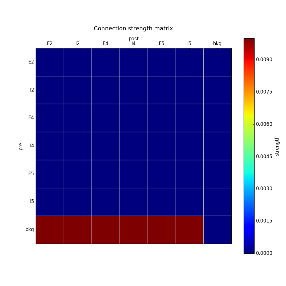
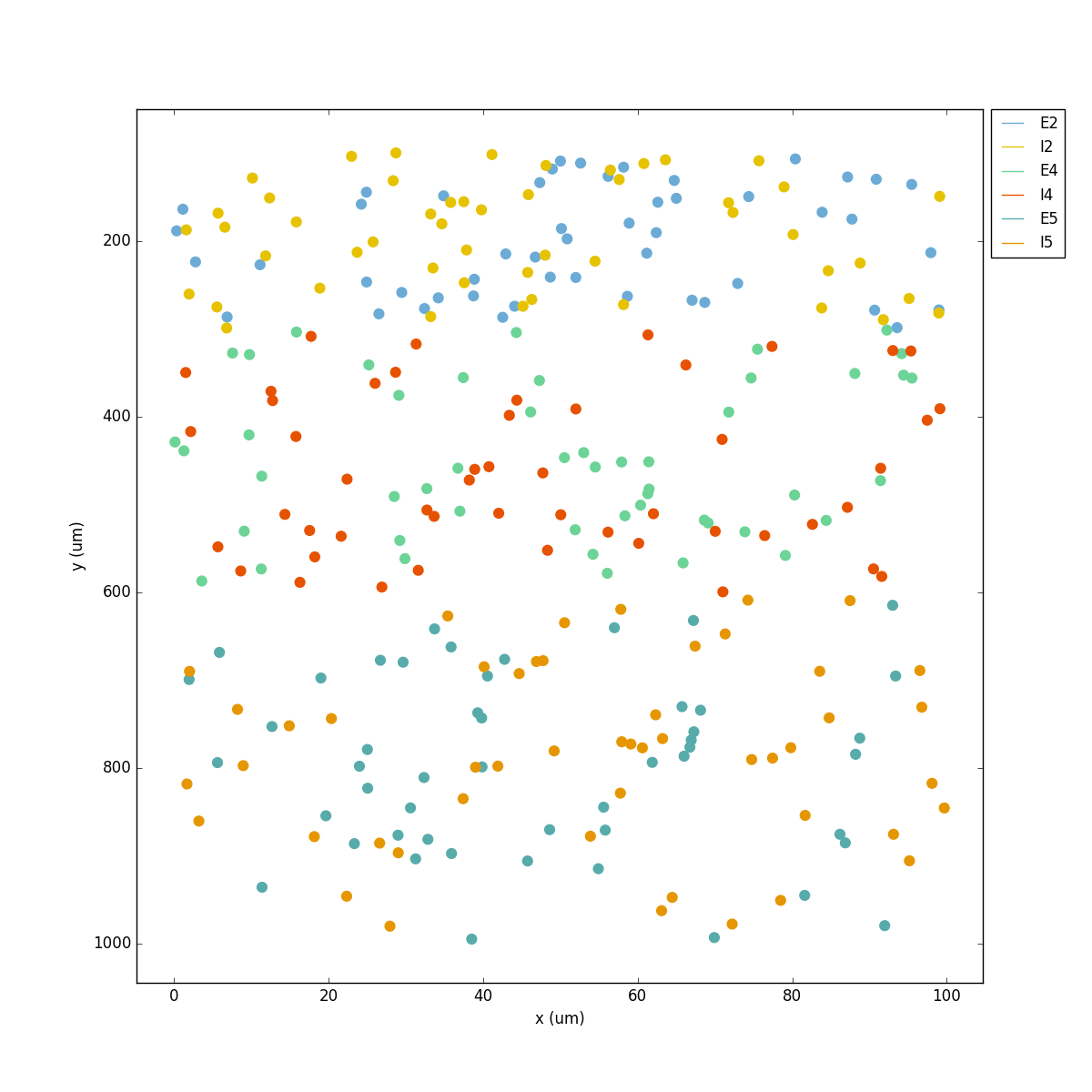
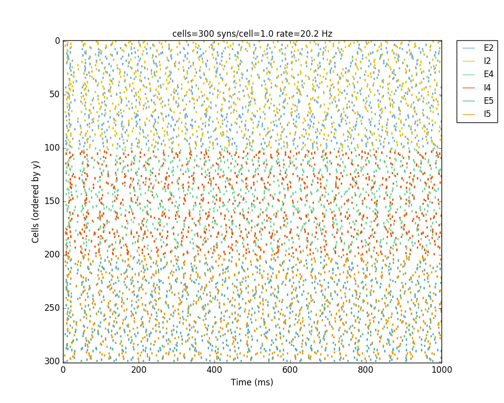
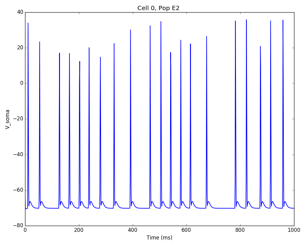
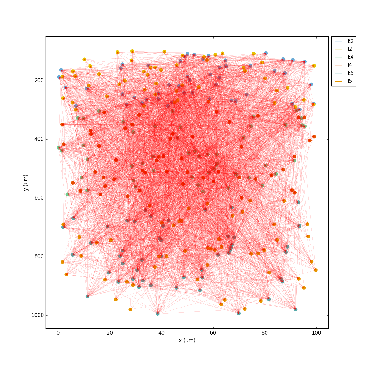
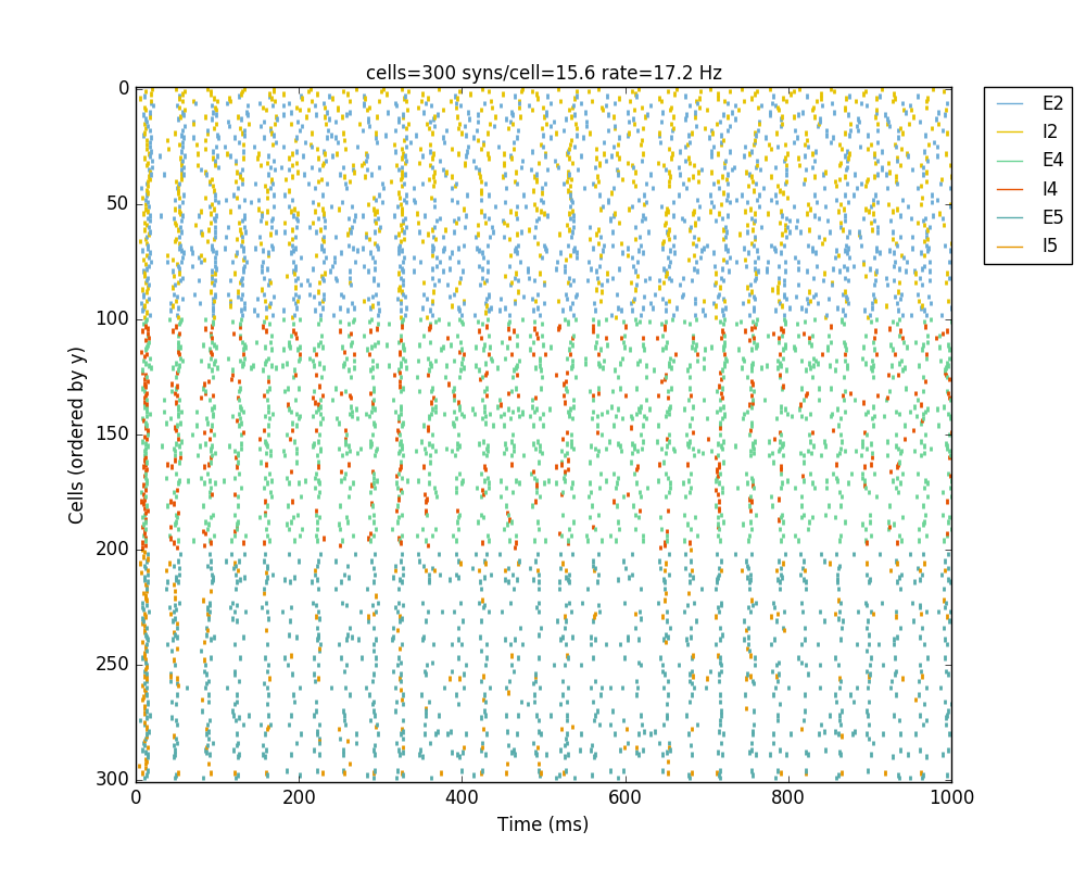
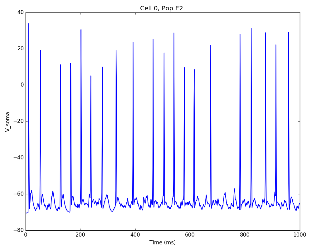
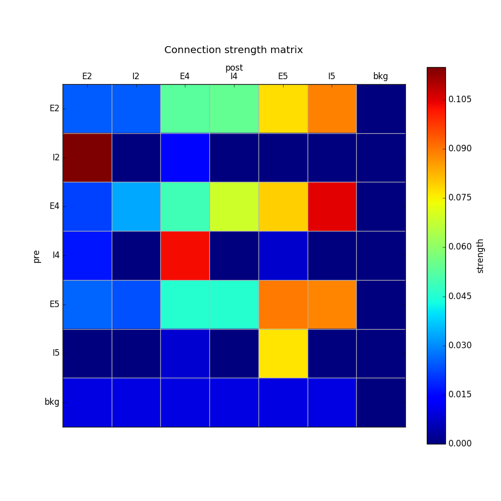
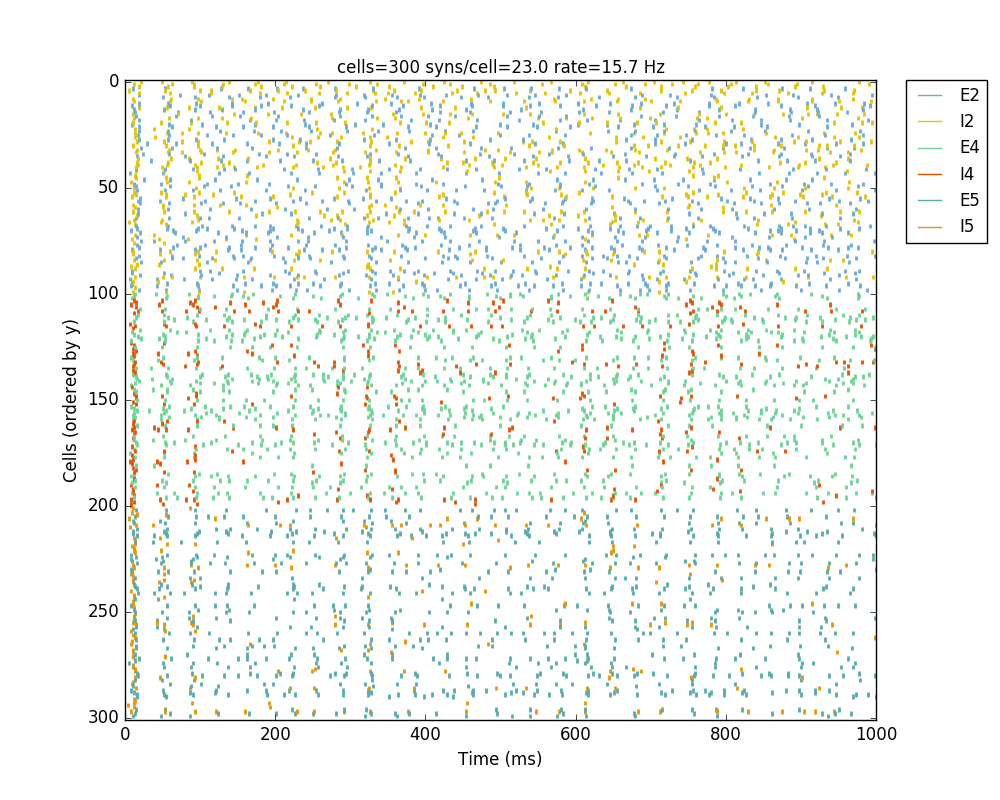
We can now add the standard simulation configuration options and the code to create and run the network. Notice that we have chosen to record and plot voltage traces of one cell in each of the excitatory populations ({'include': [('E2',0), ('E4', 0), ('E5', 5)]})), plot the raster ordered based on cell cortical depth ({'orderBy': 'y', 'orderInverse': True})), show a 2D visualization of cell positions and connections, and plot the connectivity matrix:
# Simulation options
simConfig = specs.SimConfig() # object of class SimConfig to store simulation configuration
simConfig.duration = 1*1e3 # Duration of the simulation, in ms
simConfig.dt = 0.05 # Internal integration timestep to use
simConfig.verbose = False # Show detailed messages
simConfig.recordTraces = {'V_soma':{'sec':'soma','loc':0.5,'var':'v'}} # Dict with traces to record
simConfig.recordStep = 1 # Step size in ms to save data (e.g. V traces, LFP, etc)
simConfig.filename = 'tut5' # Set file output name
simConfig.savePickle = False # Save params, network and sim output to pickle file
simConfig.analysis['plotRaster'] = {'orderBy': 'y', 'orderInverse': True, 'saveFig': True} # Plot a raster
simConfig.analysis['plotTraces'] = {'include': [('E2',0), ('E4', 0), ('E5', 5)], 'saveFig': True} # Plot recorded traces for this list of cells
simConfig.analysis['plot2Dnet'] = {'saveFig': True} # plot 2D cell positions and connections
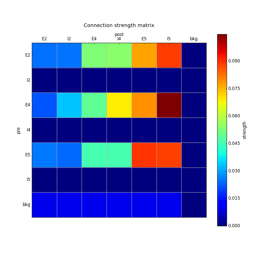
simConfig.analysis['plotConn'] = {'saveFig': True} # plot connectivity matrix
# Create network and run simulation
sim.createSimulateAnalyze(netParams = netParams, simConfig = simConfig)
If we run the model at this point we will see the cells are distributed into three layers as specified, and they all spike randomly with an average rate of 20 Hz driven by background input:
Let’s now add excitatory connections with some spatially-dependent properties to illustrate NetPyNE’s capabilities. First, let’s specify that we want excitatory cells to target all cells within a cortical depth of 100 and 1000 um, with the following code: 'postConds': {'y': [100,1000]}.
Second, let’s make the the connection weight be proportional to the cortical depth of the cell, i.e. postsynaptic cells in deeper layers will receive stronger connections than those in superficial layers. To do this we make use of the distance-related variables that NetPyNE makes available to use in string-based functions; in this case post_ynorm, which represents the normalized y location of the postsynaptic cell. For a complete list of available variables see: Functions as strings.
Finally, we can specify the delay based on the distance between the cells (dist_3D) and the propagation velocity (given as a parameter at the beginning of the code), as follows: 'delay': 'dist_3D/propVelocity'. The full code for this connectivity rules is:
netParams.connParams['E->all'] = {
  'preConds': {'cellType': 'E'}, 'postConds': {'y': [100,1000]},  #  E -> all (100-1000 um)
  'probability': 0.1 ,                  # probability of connection
  'weight': '0.005*post_ynorm',         # synaptic weight
  'delay': 'dist_3D/propVelocity',      # transmission delay (ms)
  'synMech': 'exc'}                     # synaptic mechanism
Running the model now shows excitatory connections in red, and how cells in the deeper layers (higher y values) exhibit lower rates and higher synchronization, due to increased weights leading to depolarization blockade. This difference is also visible in the voltage traces of layer 2 vs layer 5 cells:
Finally, we add inhibitory connections which will project only onto excitatory cells, specified here using the pop attribute, for illustrative purposes (an equivalent rule would be: 'postConds': {'cellType': 'E'}).
To make the probability of connection decay exponentially as a function of distance with a given length constant (probLengthConst), we can use the following distance-based expression: 'probability': '0.4*exp(-dist_3D/probLengthConst)'. The code for the inhibitory connectivity rule is therefore:
netParams.connParams['I->E'] = {                          # I -> E
        'preConds': {'cellType': 'I'},                        # presynaptic conditions
        'postConds': {'pop': ['E2','E4','E5']},               # postsynaptic conditions
        'probability': '0.4*exp(-dist_3D/probLengthConst)',   # probability of connection
        'weight': 0.001,                                      # synaptic weight
        'delay': 'dist_3D/propVelocity',                      # transmission delay (ms)
        'synMech': 'inh'}                                     # synaptic mechanism
Notice that the 2D network diagram now shows inhibitory connections in blue, and these are mostly local/lateral within layers, due to the distance-related probability restriction. These local inhibitory connections reduce the overall synchrony, introducing some richness into the temporal firing patterns of the network.


The full tutorial code for this example is available here: tut5.py.
Tutorial 6: Adding stimulation to the network
Two dictionary structures are used to specify cell stimulation parameters: stimSourceParams to define the parameters of the sources of stimulation; and stimTargetParams to specify what cells will be applied what source of stimulation (mapping of sources to cells). See Stimulation parameters for details.
In this example, we will take as a starting point the simple network in tut2.py, remove all connection parameters, and add external stimulation instead.
Below we add four typical NEURON sources of stimulation, each of a different type: IClamp, VClamp, AlphaSynapse, NetStim. Note that parameter values can also include string-based functions (Functions as strings), for example to set a uniform distribution of onset values ('onset': 'uniform(600,800)'), or maximum conductance dependent on the target cell normalized depth ('gmax': 'post_ynorm'):
netParams.stimSourceParams['Input_1'] = {'type': 'IClamp', 'del': 300, 'dur': 100, 'amp': 'uniform(0.4,0.5)'}
netParams.stimSourceParams['Input_2'] = {'type': 'VClamp', 'dur': [0,50,200], 'amp': [-60,-30,40], 'gain': 1e5, 'rstim': 1, 'tau1': 0.1, 'tau2': 0}
netParams.stimSourceParams['Input_3'] = {'type': 'AlphaSynapse', 'onset': 'uniform(300,600)', 'tau': 5, 'gmax': 'post_ynorm', 'e': 0}
netParams.stimSourceParams['Input_4'] = {'type': 'NetStim', 'interval': 'uniform(20,100)', 'number': 1000, 'start': 600, 'noise': 0.1}
Now we can map or apply any of the above stimulation sources to any subset of cells in the network by adding items to the stimTargetParams dict. Note that we can use any of the cell tags (e.g. ‘pop’, ‘cellType’ or ‘ynorm’) to select which cells will be stimulated. Additionally, using the ‘cellList’ option, we can target a specific list of cells (using relative cell ids) within the subset of cells selected (e.g. first 15 cells of the ‘S’ population):
netParams.stimTargetParams['Input_1->S'] = {'source': 'Input_1', 'sec':'soma', 'loc': 0.8, 'conds': {'pop':'S', 'cellList': range(15)}}
netParams.stimTargetParams['Input_2->S'] = {'source': 'Input_2', 'sec':'soma', 'loc': 0.5, 'conds': {'pop':'S', 'ynorm': [0,0.5]}}
netParams.stimTargetParams['Input_3->M1'] = {'source': 'Input_3', 'sec':'soma', 'loc': 0.2, 'conds': {'pop':'M', 'cellList': [2,4,5,8,10,15,19]}}
netParams.stimTargetParams['Input_4->PYR'] = {'source': 'Input_4', 'sec':'soma', 'loc': 0.5, 'weight': '0.1+normal(0.2,0.05)','delay': 1, 'conds': {'cellType':'PYR', 'ynorm': [0.6,1.0]}}
Note
The stimTargetParams of NetStims require connection parameters (e.g. weight and delay), since a new connection will be created to map/apply the NetStim to each target cell.
Note
NetStims can be added both using the above method (as stims), or by creating a population with 'cellModel': 'NetStim' and adding the appropriate connections.
Running the above network with different types of stimulation should produce the following raster:
The full tutorial code for this example is available here: tut6.py.
Tutorial 7: Modifying the instantiated network interactively
This example is directed at the more experienced users who might want to interact directly with the NetPyNE generated structure containing the network model and NEURON objects. We will model a Hopfield-Brody network where cells are connected all-to-all and firing synchronize due to mutual inhibition (inhibition from other cells provides a reset, locking them together). The level of synchronization depends on the connection weights, which we will modify interactively.
We begin by creating a new file (tut7.py) describing a simple network with one population (hop) of 50 cells and background input of 50 Hz (similar to the previous simple tutorial example tut2.py). We create all-to-all inhibitory connections within the hop population, but set the weights to 0 initially:
from netpyne import specs

###############################################################################
# NETWORK PARAMETERS
###############################################################################

netParams = specs.NetParams()  # object of class NetParams to store the network parameters

# Cell parameters
## PYR cell properties
secs = {}
secs['soma'] = {'geom': {}, 'topol': {}, 'mechs': {}}
secs['soma']['geom'] = {'diam': 18.8, 'L': 18.8}
secs['soma']['mechs']['hh'] = {'gnabar': 0.12, 'gkbar': 0.036, 'gl': 0.003, 'el': -70}
netParams.cellParams['PYR'] = {'secs': secs}  # add dict to list of cell properties

# Population parameters
netParams.popParams['hop'] = {'cellType': 'PYR', 'cellModel': 'HH', 'numCells': 50}      # add dict with params for this pop
#netParams.popParams['background'] = {'cellModel': 'NetStim', 'rate': 50, 'noise': 0.5}  # background inputs

# Synaptic mechanism parameters
netParams.synMechParams['exc'] = {'mod': 'Exp2Syn', 'tau1': 0.1, 'tau2': 1.0, 'e': 0}
netParams.synMechParams['inh'] = {'mod': 'Exp2Syn', 'tau1': 0.1, 'tau2': 1.0, 'e': -80}

# Stimulation parameters
netParams.stimSourceParams['bkg'] = {'type': 'NetStim', 'rate': 50, 'noise': 0.5}
netParams.stimTargetParams['bkg->all'] = {'source': 'bkg', 'conds': {'pop': 'hop'}, 'weight': 0.1, 'delay': 1, 'synMech': 'exc'}

# Connectivity parameters
netParams.connParams['hop->hop'] = {
        'preConds': {'pop': 'hop'},         # presynaptic conditions
        'postConds': {'pop': 'hop'},        # postsynaptic conditions
        'weight': 0.0,                      # weight of each connection
        'synMech': 'inh',                   # target inh synapse
        'delay': 5}                         # delay
We now add the standard simulation configuration options, and include the syncLines option so that raster plots show vertical lines at each spike as an indication of synchrony:
###############################################################################
# SIMULATION PARAMETERS
###############################################################################
simConfig = specs.SimConfig()  # object of class SimConfig to store simulation configuration

# Simulation options
simConfig.duration = 0.5*1e3        # Duration of the simulation, in ms
simConfig.dt = 0.025                # Internal integration timestep to use
simConfig.verbose = False           # Show detailed messages
simConfig.recordTraces = {'V_soma':{'sec':'soma','loc':0.5,'var':'v'}}  # Dict with traces to record
simConfig.recordStep = 1            # Step size in ms to save data (eg. V traces, LFP, etc)
simConfig.filename = 'model_output' # Set file output name
simConfig.savePickle = False        # Save params, network and sim output to pickle file

simConfig.analysis['plotRaster'] = {'syncLines': True, 'saveFig': True}      # Plot a raster
simConfig.analysis['plotTraces'] = {'include': [1], 'saveFig': True}         # Plot recorded traces for this list of cells
simConfig.analysis['plot2Dnet'] = {'saveFig': True}                          # plot 2D cell positions and connections
Finally, we add the code to create the network and run the simulation, but for illustration purposes, we use the individual function calls for each step of the process (instead of the all-encompassing sim.createAndSimulate() function used before):
###############################################################################
# EXECUTION CODE (via netpyne)
###############################################################################
from netpyne import sim

# Create network and run simulation
sim.initialize(                     # create network object and set cfg and net params
        simConfig = simConfig,          # pass simulation config and network params as arguments
        netParams = netParams)
sim.net.createPops()                # instantiate network populations
sim.net.createCells()               # instantiate network cells based on defined populations
sim.net.connectCells()              # create connections between cells based on params
sim.net.addStims()                  # add stimulation
sim.setupRecording()                # setup variables to record for each cell (spikes, V traces, etc)
sim.runSim()                        # run parallel Neuron simulation
sim.gatherData()                    # gather spiking data and cell info from each node
sim.saveData()                      # save params, cell info and sim output to file (pickle,mat,txt,etc)
sim.analysis.plotData()             # plot spike raster
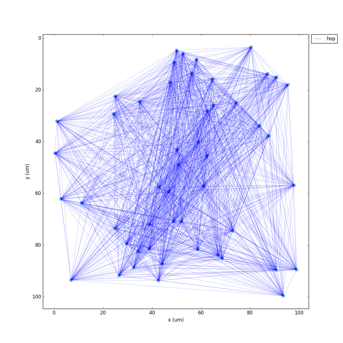
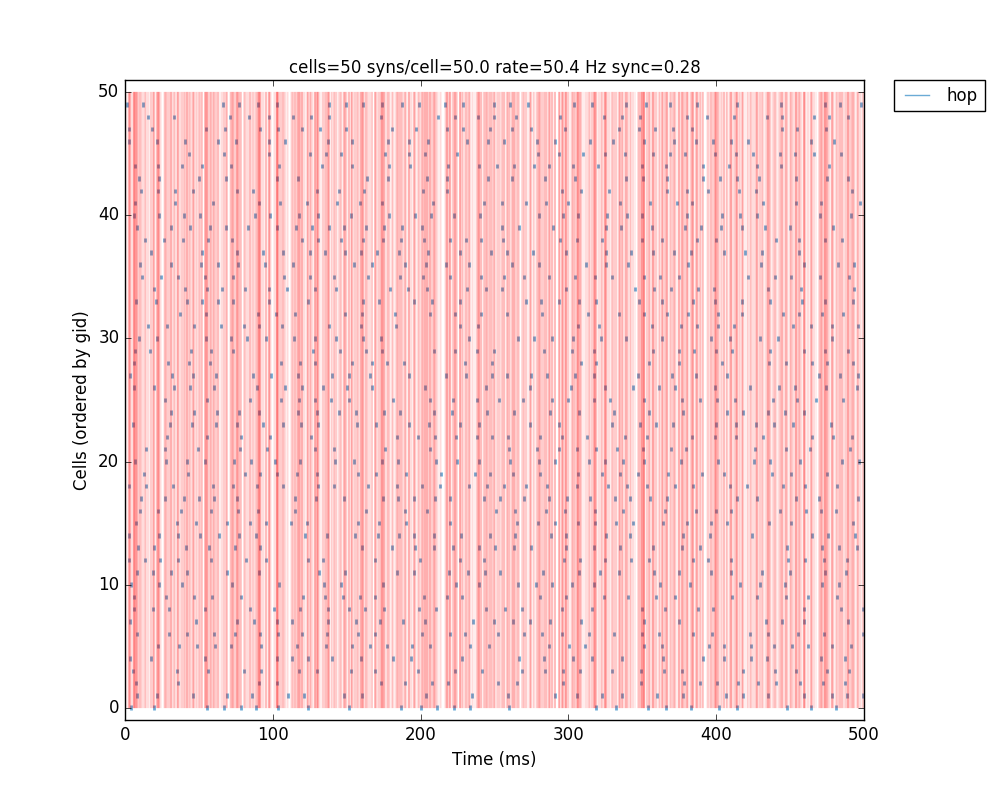
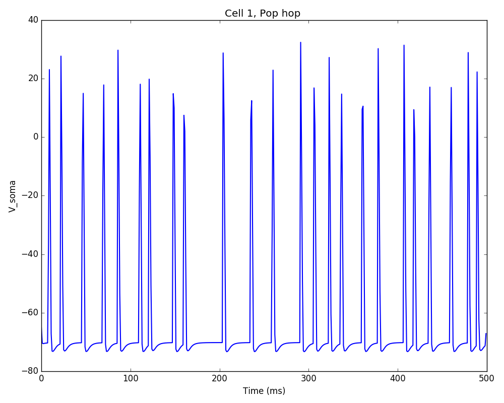
If we run the above code, the resulting network 2D map shows the inhibitory connections in blue, although these don’t yet have any effect since the weight is 0. The raster plot shows random firing driven by the 50 Hz background inputs, and a low sync measure of 0.26 (vertical red lines illustrate poor synchrony):
Note
We can now access the instantiated network with all the cell and connection metadata, as well as the associated NEURON objects (Sections, Netcons, etc.). The sim object contains a net object which, in turn, contains a list of Cell objects called cells. Each Cell object contains a structure with its tags (tags), sections (secs), connections (conns), and external inputs (stims). NEURON objects are contained within this python hierarchical structure. See NetPyNE data model (structure of instantiated network and output data) for details.
Note
A list of population objects is available via sim.net.pops; each object will contain a list cellGids with all gids of cells belonging to this populations, and a dictionary tags with population properties.
Note
Spiking data is available via sim.allSimData['spkt'] and sim.allSimData['spkid']. Voltage traces are available via e.g. sim.allSimData['V']['cell_25'] (for cell with gid 25).
Note
All the simulation configuration options can be modified interactively via sim.cfg. For example, to turn off plotting of 2D visualization, run: sim.cfg.analysis['plot2Dnet']=False
A representation of the instantiated network structure generated by NetPyNE is shown below:
The Network object net also provides functions to easily modify its cell, connection and stimulation parameters: modifyCells(params), modifyConns(params) and modifyStims(params), respectively. The syntax for the params argument is similar to that used to initially set the network parameters, i.e. a dictionary including the conditions and parameters to set. For details see Network class methods.
We can therefore call the sim.net.modifyConns() function to increase all the weights of the inhibitory connections (e.g. to 0.5), and then rerun the simulation interactively:
###############################################################################
# INTERACTING WITH INSTANTIATED NETWORK
###############################################################################

# modify conn weights
sim.net.modifyConns({'conds': {'label': 'hop->hop'}, 'weight': 0.5})

sim.runSim()                          # run parallel Neuron simulation
sim.gatherData()                      # gather spiking data and cell info from each node
sim.saveData()                        # save params, cell info and sim output to file (pickle,mat,txt,etc)
sim.analysis.plotData()               # plot spike raster
Note
that for the condition we have used the hop->hop label, which makes reference to the set of recurrent connections previously created.
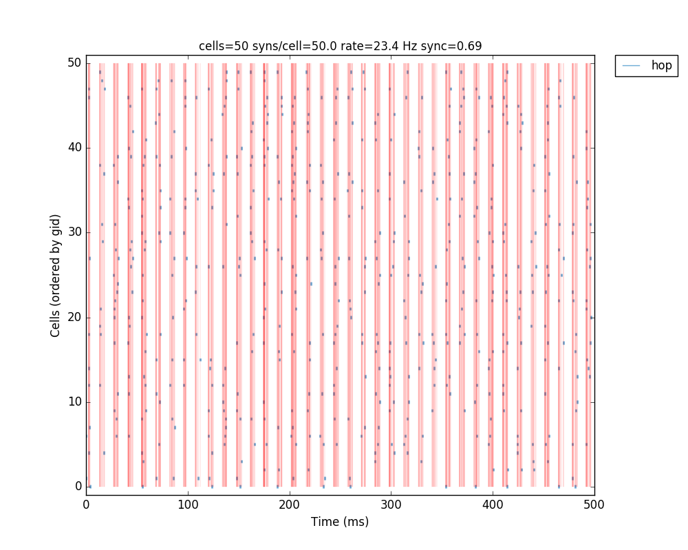
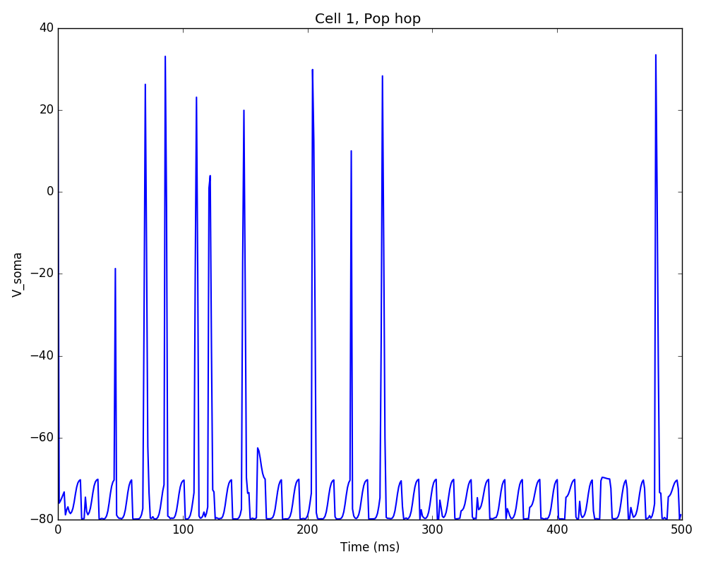
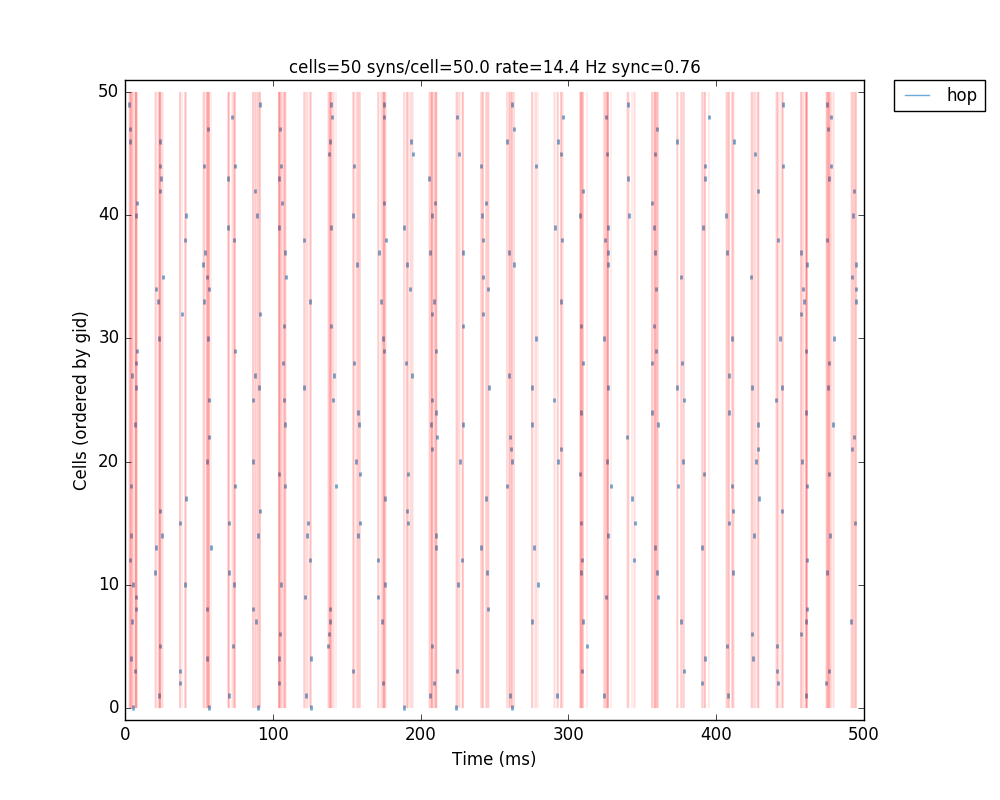
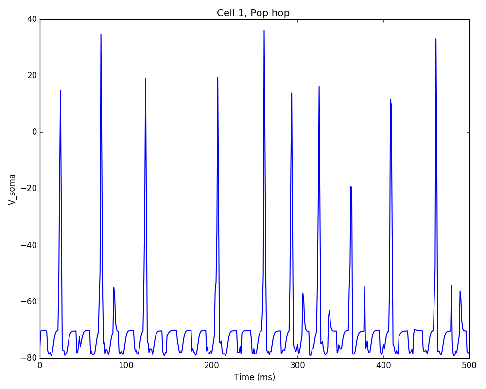
The resulting plots show that the increased mutual inhibition synchronizes the network activity, increasing the synchrony measure to 0.69:
Additionally, we could also modify some of the cell properties to observe how this affects synchrony. The code below modifies the soma length of all cells in the ‘hop’ population to 160 um:
# modify cells geometry
sim.net.modifyCells({'conds': {'pop': 'hop'},
                    'secs': {'soma': {'geom': {'L': 160}}}})

sim.simulate()
sim.analysis.plotRaster(syncLines=True)
sim.analysis.plotTraces(include = [1])
Note
For illustration purposes we make use of the sim.simulate() wrapper, which simply calls runSim() and gatherData(). Additionally, we interactively call the sim.plotRaster() and sim.plotTraces() functions.
The resulting plot shows decreased firing rate and increased synchrony due to the new cell geometry:
The full tutorial code for this example is available here: tut7.py.
Tutorial 8: Running batch simulations
Here we are going to illustrate how to run batch simulations using the simple network in Tutorial 2. By batch simulations we mean modifying some parameter values within a given range and automatically running simulations for all combinations of these parameter values (also known as grid parameter search).
The first thing we need to do is break up the tut2.py code into three different files – although not needed for such small models, this will be very helpful for more larger, more complex models. The file organization should be as follows (click on filename to download):
tut8_netParams.py: Defines the network model (netParams object). Includes “fixed” parameter values of cells, synapses, connections, stimulation, etc. Changes to this file should only be made for relatively stable improvements of the model. Parameter values that will be varied systematically to explore or tune the model should be included here by referencing the appropiate variable in the simulation configuration (cfg) module. Only a single netParams file is required for each batch of simulations.tut8_cfg.py: Simulation configuration (simConfig object). Includes parameter values for each simulation run such as duration, dt, recording parameters etc. Also includes the model parameters that are being varied to explore or tune the network. When running a batch, NetPyNE will automatically create one cfg file for each parameter configuration (using this one as a starting point).tut8_init.py: Sequence of commands to run a single simulation. Can be executed via ‘python init.py’. When running a batch, NetPyNE will call init.py multiple times and pass a different cfg file for each of the parameter configurations explored.
We will also need to add a new file to control the batch simulation:
tut8_batch.py: Defines the parameters and parameter values to be explored in a batch of simulations, the run configuration (e.g. whether to use MPI+Bulletin Board (for multicore machines) or SLURM/PBS Torque (for HPCs)), and the command to run the batch.
In summary, netParams.py for fixed (network) parameters, cfg.py for variable (simulation) parameters, init.py to run a simulation, and batch.py to run a batch of simulations exploring combinations of parameter values.
Lets say we want to explore how the connection weight and the synaptic decay time constant affect the firing rate of the motor population. The first step would be to modify tut8_netParams.py so these parameters are variable, i.e. different in each simulation. Therefore, we will change them from having fixed values (e.g. 5.0 and 0.01) to depending on a variable from simConfig: cfg.synMechTau2 and cfg.connWeight (note that for simplicity we renamed simConfig to cfg):
...

## Synaptic mechanism parameters
netParams.synMechParams['exc'] = {'mod': 'Exp2Syn', 'tau1': 0.1, 'tau2': cfg.synMechTau2, 'e': 0}  # excitatory synaptic mechanism

...

## Cell connectivity rules
netParams.connParams['S->M'] = {    #  S -> M label
        'preConds': {'pop': 'S'},       # conditions of presyn cells
        'postConds': {'pop': 'M'},      # conditions of postsyn cells
        'probability': 0.5,             # probability of connection
        'weight': cfg.connWeight,       # synaptic weight
        'delay': 5,                     # transmission delay (ms)
        'synMech': 'exc'}               # synaptic mechanism
Therefore, this also requires changing tut8_netParams.py to import the cfg module so that these two variables are available. The code will first attempt to load the cfg module from __main__, which refers to the parent module which was initially executed by the user, in this case, tut8_init.py. As mentioned before, tut8_init.py is responsible for loading both netParams and cfg and running the simulation. If that fails, the code will load cfg directly from the tut8_cfg.py file. To implement this we will add the following lines at the beginning of tut8_netParams.py:
try:
        from __main__ import cfg  # import SimConfig object with params from parent module
except:
        from tut8_cfg import cfg  # if no simConfig in parent module, import directly from tut8_cfg module
The next step is to add these two variables to the tut8_cfg.py so that they exist and can be used by netParams and modified in the batch simulation:
# Variable parameters (used in netParams)
cfg.synMechTau2 = 50
cfg.connWeight = 0.01
Note we will also add to tut8_cfg.py the following line so that the average firing rates of each populations are printed in screen and saved to the output file:
cfg.printPopAvgRates = True
The tut8_init.py will contain only three lines, and just one new line compared to tut2.py. This new line calls the method readCmdLineArgs which takes care of reading arguments from the command line. This is required to run the batch simulations, since NetPyNE will create multiple cfg files with the different parameter combinations and run them using command line arguments of the form: python tut8_init.py simConfig=filepath netParams=filepath. You do not need to worry about this, since this is done behind the scenes by NetPyNE. The tut8_init.py should look like this:
from netpyne import sim

# read cfg and netParams from command line arguments if available; otherwise use default
simConfig, netParams = sim.readCmdLineArgs(simConfigDefault='tut8_cfg.py', netParamsDefault='tut8_netParams.py')

# Create network and run simulation
sim.createSimulateAnalyze(netParams=netParams, simConfig=simConfig)
At this point you can run the simulation using e.g. python tut8_init.py and it should produce the same result as in Tutorial 2 (tut2.py).
Now we will add the tut8_batch.py which contains all the information related to the batch simulations. We have defined a function batchTauWeight to explore this specific combination of parameters. We could later define other similar functions to create other batches.
The first thing we do is create an ordered dictionary params – this will be of a special NetPyNE type (specs.ODict) but it essentially behaves like an ordered dictionary. Next we add the parameters to explore as keys of this dictionary – synMechTau2 and connWeight – and add the list of parameter values to try in the batch simulation as the dictionary keys – [3.0, 5.0, 7.0] and [0.005, 0.01, 0.15]. Note that parameter names should coincide with the variables defined in cfg.
We then create an object b of the NetPyNE class Batch and pass as arguments the parameters to explore, and the files containing the netParams and simConfig modules. Finally, we customize some attributes of the Batch object, including the the batch label ('tauWeight'), used to create the output file; the folder where to save the data ('tut8_data'), the method used to explore parameters ('grid'), meaning all combinations of the parameter values; and the run configuration indicating we want to use 'mpi' (this uses MPI and NEURON’s Bulletin Board; other options are available for supercomputers), the 'tut8_init.py' to run each sims, and to 'skip' runs if the output files already exist.
At the end we just need to add the command to launch the batch simulation: b.run().
The tut8_batch.py should look like this:
from netpyne import specs
from netpyne.batch import Batch

def batchTauWeight():
        # Create variable of type ordered dictionary (NetPyNE's customized version)
        params = specs.ODict()

        # fill in with parameters to explore and range of values (key has to coincide with a variable in simConfig)
        params['synMechTau2'] = [3.0, 5.0, 7.0]
        params['connWeight'] = [0.005, 0.01, 0.15]

        # create Batch object with parameters to modify, and specifying files to use
        b = Batch(params=params, cfgFile='tut8_cfg.py', netParamsFile='tut8_netParams.py',)

        # Set output folder, grid method (all param combinations), and run configuration
        b.batchLabel = 'tauWeight'
        b.saveFolder = 'tut8_data'
        b.method = 'grid'
        b.runCfg = {'type': 'mpi',
                                'script': 'tut8_init.py',
                                'skip': True}

        # Run batch simulations
        b.run()

# Main code
if __name__ == '__main__':
        batchTauWeight()
To run the batch simulations you will need to have MPI properly installed and NEURON configured to use MPI. Run the following command: mpiexec -np [num_cores] nrniv -python -mpi tut8_batch.py , where [num_cores] should be replaced with the number of processors you want to use. The minimum required is 2, since one will be used to schedule the jobs (master node); e.g. if you select 4 processors, one will be used to schedule jobs, and the other 3 will run NEURON simulations with different parameter combinations.
Once the simulations are complete you should have a new folder tut8_data with the following files:
tauWeight_netParams.py: a copy of the original netParams file used (
tut8_netParams.py)tauWeight_batchScript.py: a copy of the original batch file used (
tut8_batch.py)tauWeight_batch.json: a JSON file with the batch parameters and run option used.
For each combination of parameters (with x, y representing the indices of the parameter values):
tauWeight_x_y_cfg.json: JSON file with all the
cfgvariables copied fromtut8_cfg.pybut with the values ofsynMechTau2andconnWeightfor this specific combination of batch parameters.tauWeight_x_y.json: JSON file with the output data for this combination of batch parameters; output data will contain by default the
netParams,net,simConfigandsimData.tauWeight_x_y_raster.png and tauWeight_x_y_traces.png: output figures for this combination of parameters.
To analyze the output data you can download tut8_analysis.py. This file has functions to read and plot a matrix showing the results from the batch simulations. This file requires the Pandas and Seaborn packages.
Note
The analysis functions in (tut8_analysis.py) will be soon integrated into NetPyNE, and so we won’t go into the details of the code.
Running python tut8_analysis.py should produce a color plot showing the relation between the two parameters explored and the firing rate of the M populations:
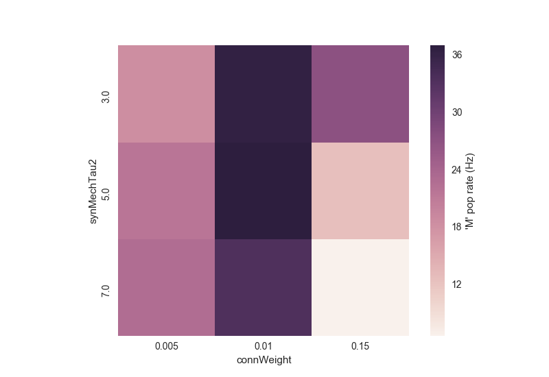
Notice how the rate initially increases as a function of connection weight, but then decreases due to depolarization blockade; and how the effect of the synaptic time decay constant (synMechTau2) depends on whether the cell is spiking normally or in blockade. Batch simulations and analyses facilitate exploration and understanding of these complex interactions.
Note
For the more advanced users, this is what NetPyNE does under the hood when you run a batch:
Copy netParams.py (or whatever file is specified) to batch data folder
Load cfg (SimConfig object) from cfg.py (or whatever file is specified)
Iterate parameter combinations:
3a) Modify cfg (SimConfig object) with the parameter values
3b) Save cfg to .json file
3c) Run simulation by passing netParams.py and cfg.json files as arguments; this means the code in netParams.py is executed each time but cfg is just a set of fixed saved values.
See also
The full description of options available in the Batch class will be available soon in the User Documentation.
Tutorial 9: Recording and plotting LFPs
Examples of how to record and analyze local field potentials (LFP) in single cells and networks are included in the examples folder: LFP recording example . LFP recording also works with parallel simulations.
To record LFP just set the list of 3D locations of the LFP electrodes in the simConfig attribute recordLFP e.g. simConfig.recordLFP = e.g. [[50, 100, 50], [50, 200, 50]] (note the y coordinate represents depth, so will be represented as a negative value when plotted). The LFP signal in each electrode is obtained by summing the extracellular potential contributed by each segment of each neuron. Extracellular potentials are calculated using the “line source approximation” and assuming an Ohmic medium with conductivity sigma = 0.3 mS/mm. For more information on modeling LFPs see Scholarpedia or this article .
The recorded LFP signal will be stored in sim.allSimData['LFP'] as a 2D list of size timeSteps * numElectrodes e.g. sim.allSimData[‘LFP’][10][2]` corresponds to the LFP value of electrode 2 at time step 10. It is possible to record the LFP signal generated by each individual cell by setting simConfig.saveLFPCells = True – this will be stored in sim.allSimData['LFPCells'] as a 3D list with size cells * timeSteps * numElectrodes.
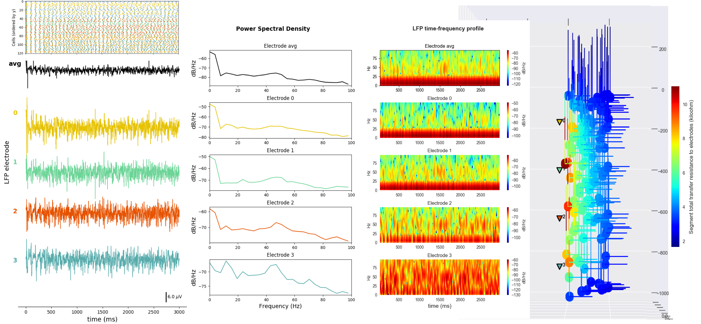
To plot the LFP use the sim.analysis.plotLFP() method. This allows to plot for each electrode: 1) the time-resolved LFP signal (‘timeSeries’), 2) the power spectral density (‘PSD’), 3) the spectrogram / time-frequency profile (‘spectrogram’), 4) and the 3D locations of the electrodes overlaid over the model neurons (‘locations’). See Analysis-related functions for the full list of plotLFP() arguments.
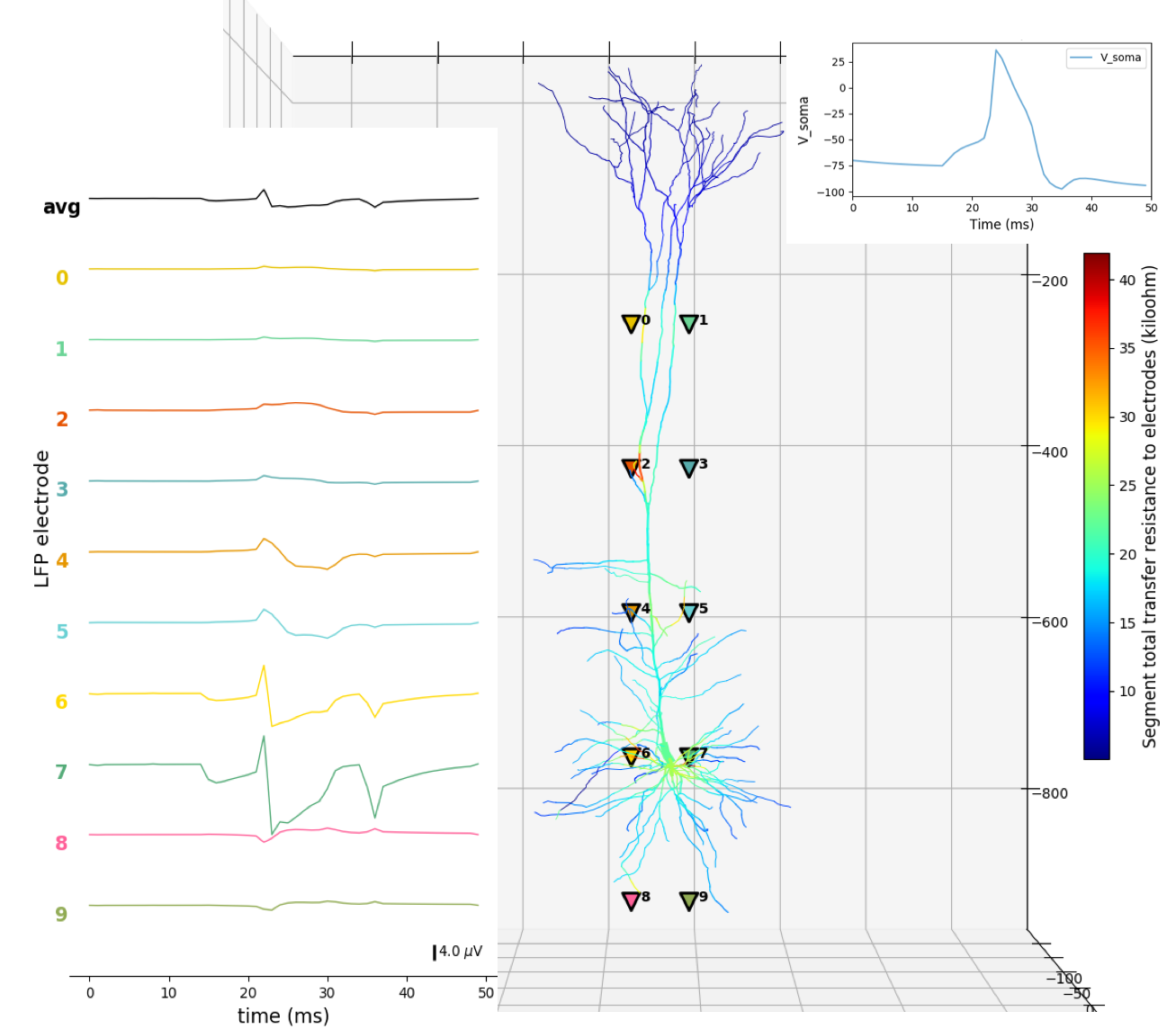
The first example shows LFP recording for a single cell – M1 corticospinal neuron – with 700+ compartments (segments) and multiple somatic and dendritic ionic channels. The cell parameters are loaded from a .json file. The cell receives NetStim input to its soma via an excitatory synapse. Ten LFP electrodes are placed at both sides of the neuron at 5 different cortical depths. The soma voltage, LFP time-resolved signal and the 3D locations of the electrodes are plotted:
The second example shows LFP recording for a network very similar to that shown in Tutorial 5. However, in this case, the cells have been replaced with a more realistic model: a 6-compartment M1 corticostriatal neuron with multiple ionic channels. The cell parameters are loaded from a .json file. Cell receive NetStim inputs and include excitatory and inhibitory connections. Four LFP electrodes are placed at different cortical depths. The raster plot and LFP time-resolved signal, PSD, spectrogram and 3D locations of the electrodes are plotted:
Tutorial 10: Network with Reaction-Diffusion (RxD)
NetPyNE’s high-level specifications also supports NEURON’s reaction-diffusion (RxD) components. RxD enables to specify the diffusion of molecules (egcalcium, potassium or IP3) intracellularly, subcellularly (by including organelles such as endoplasmic reticulum and mitochondria), and extracellularly is the context of signaling and enzymatic processing – egmetabolism, phosphorylation, buffering, second messenger cascades. This helps to couple molecular-level chemophysiology to the classical electrophysiology at subcellular, cellular and network scales.
The netParams.rxdParams dictionary can be used to define the different RxD components: regions, species, states, reactions, multicompartmentReactions and rates. Example models that include RxD components in single cells and networks are included in the examples folder: RxD buffering example and RxD network example. RxD also works with parallel simulations.
See also
For a comprehensive description of all the features available in NetPyNE see User Documentation.