User Documentation
Model components and structure
Creating a network model requires:
An object
netParamsof classspecs.NetParamswith the network parameters.An object
simConfigof classspecs.SimConfigwith the simulation configuration options.A call to the method(s) to create and run the network model, passing as arguments the above dictionaries, e.g.
createSimulateAnalyze(netParams, simConfig).
These components can be included in a single or multiple Python files. This section comprehensively describes how to define the network parameters and simulation configuration options, as well as the methods available to create and run the network model.
Network parameters
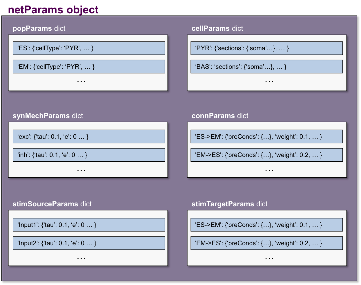
The netParams object of class NetParams includes all the information necessary to define your network. It is composed of the following ordered dictionaries:
cellParams- cell types and their associated parameters (e.g. cell geometry)popParams- populations in the network and their parameterssynMechParams- synaptic mechanisms and their parametersconnParams- network connectivity rules and their associated parameters.subConnParams- network subcellular connectivity rules and their associated parameters.stimSourceParams- stimulation sources parameters.stimTargetParams- mapping between stimulation sources and target cells.rxdParams- reaction-diffusion (RxD) components and their parameters.
Each of these ordered dicts can be filled in directly or using the NetParams object methods. Both ways are equivalent, but the object methods provide checks on the syntax of the parameters being added. Below are two equivalent ways of adding an item to the popParams ordered dictionary:
from netpyne import specs
netParams = specs.NetParams()

# Method 1: direct
netParams.popParams['Pop1'] = {'cellType': 'PYR', 'numCells': 20}

# Method 2: using object method
netParams.addPopParams(label='Pop1', params={'cellType': 'PYR', 'numCells': 20})
The organization of netParams is consistent with the standard sequence of events that the framework executes internally:
sets the cell properties according to type based on
cellParamscreates a
Networkobject and adds inside it a set ofCellandPopulationobjects based onpopParamscreates a set of connections based on
connParamsandsubConnParams(checking which presynpatic and postsynaptic cells match the connection rule conditions), and using the synaptic parameters insynMechParamsadds stimulation to the cells based on
stimSourceParamsandstimTargetParams
Additionally, netParams contains the following customizable single-valued attributes (e.g. netParams.sizeX = 100):
scale: Scale factor multiplier for number of cells (default: 1)
shape: Shape of network: ‘cuboid’, ‘cylinder’ or ‘ellipsoid’ (default: ‘cuboid’)
sizeX: x-dimension (horizontal length) network size in um (default: 100)
sizeY: y-dimension (vertical height or cortical depth) network size in um (default: 100)
sizeZ: z-dimension (horizontal depth) network size in um (default: 100)
rotateCellsRandomly: Random rotation of cells around y-axis [min,max] radians, e.g. [0, 3.0] (default: False)
defaultWeight: Default connection weight (default: 1)
defaultDelay: Default connection delay, in ms (default: 1)
propVelocity: Conduction velocity in um/ms (e.g. 500 um/ms = 0.5 m/s) (default: 500)
scaleConnWeight: Connection weight scale factor (excludes NetStims) (default: 1)
scaleConnWeightNetStims: Connection weight scale factor for NetStims (default: 1)
scaleConnWeightModels: Connection weight scale factor for each cell model, e.g. {‘HH’: 0.1, ‘Izhi’: 0.2} (default: {})
popTagsCopiedToCells: List of tags that will be copied from the population to the cells (default: [‘pop’, ‘cellModel’, ‘cellType’])
Other arbitrary entries to the netParams dict can be added and used in custom-defined functions for connectivity parameters (see Functions as strings).
Cell types
Each item of the cellParams ordered dictionary consists of a key and a value. The key is a label to identify this cell type. The value consists of a dictionary that defines the cell properties, containing the following fields:
secs - Dictionary containing the sections of the cell, each in turn containing the following fields (can omit those that are empty):
- geom: Dictionary with geometry properties, such as
diam,LorRa. Can optionally include a field
pt3dwith a list of 3D points, each defined as a tuple of the form(x,y,z,diam)Values ofdiam,LorRacan be defined as functions (see Functions as strings).
- geom: Dictionary with geometry properties, such as
- topol: Dictionary with topology properties.
Includes
parentSec(label of parent section),parentX(parent location where to make connection) andchildX(current section –child– location where to make connection).
- mechs: Dictionary of density/distributed mechanisms.
The key contains the name of the mechanism (e.g. ‘hh’ or ‘pas’) The value contains a dictionary with the properties of the mechanism (e.g.
{'g': 0.003, 'e': -70}). These properties can be defined as functions (see Functions as strings).
- ions: Dictionary of ions.
The key contains the name of the ion (e.g. ‘na’ or ‘k’) The value contains a dictionary with the properties of the ion for the particular section (e.g.
{'e': -70}). Properties available are'e': reversal potential,'i': internal concentration of the ion at that section, and'o': the extracellular concentration of the ion at that section.
- pointps: Dictionary of point processes (excluding synaptic mechanisms).
The key contains an arbitrary label (e.g. ‘Izhi’) The value contains a dictionary with the point process properties (e.g.
{'mod':'Izhi2007a', 'a':0.03, 'b':-2, 'c':-50, 'd':100, 'celltype':1}). These properties can be defined as functions (see Functions as strings).Apart from internal point process variables, the following properties can be specified for each point process:
mod,the name of the NEURON mechanism, e.g.'Izhi2007a'loc, section location where to place synaptic mechanism, e.g.1.0, default=0.5vref(optional), internal mechanism variable containing the cell membrane voltage, e.g.'V'synList(optional), list of internal mechanism synaptic mechanism labels, e.g. [‘AMPA’, ‘NMDA’, ‘GABAB’]
vinit - (optional) Initial membrane voltage (in mV) of the section (default: -65)
e.g.
cellRule['secs']['soma']['vinit'] = -72spikeGenLoc - (optional) Indicates that this section is responsible for spike generation (instead of the default ‘soma’), and provides the location (segment) where spikes are generated.
e.g.
cellRule['secs']['axon']['spikeGenLoc'] = 1.0threshold - (optional) Threshold voltage (in mV) used to detect a spike originating in this section of the cell. If omitted, defaults to
netParams.defaultThreshold = 10.0
e.g.
cellRule['secs']['soma']['threshold'] = 5.0secLists - (optional) Dictionary of sections lists (e.g. {‘all’: [‘soma’, ‘dend’]})
- vars - (optional) Dictionary of user-defined variables that can be referenced in properties of any section of this cell type.
Example of usage:
cellRule['secs']['dend1']['mechs']['pas'] = {'g': 'g_default + 1e-6'}  # cell variable 'g_default' referenced
cellRule['secs']['dend2']['mechs']['pas'] = {'g': 'g_default + 1.5e-6'}  # cell variable 'g_default' referenced
cellRule['vars'] = {'g_default': 0.0000357} # cell variable 'g_default' defined
Values of cell variables themselves can also be defined as functions (see Functions as strings), e.g.
cellRule['vars'] = {'g_default': 'normal(3.57e-5, 1e-7)}
Example of adding two different cell types:
## PYR_HH cell properties
soma = {'geom': {}, 'mechs': {}}  # soma properties
soma['geom'] = {'diam': 18.8, 'L': 18.8, 'Ra': 123.0, 'pt3d': []}
soma['geom']['pt3d'].append((0, 0, 0, 20))
soma['geom']['pt3d'].append((0, 0, 20, 20))
soma['mechs']['hh'] = {'gnabar': 0.12, 'gkbar': 0.036, 'gl': 0.003, 'el': -70}

dend = {'geom': {}, 'topol': {}, 'mechs': {}}  # dend properties
dend['geom'] = {'diam': 5.0, 'L': 150.0, 'Ra': 150.0, 'cm': 1}
dend['topol'] = {'parentSec': 'soma', 'parentX': 1.0, 'childX': 0}
dend['mechs']['pas'] = {'g': 0.0000357, 'e': -70}

PYR_HH_dict = {'secs': {'soma': soma, 'dend': dend}}
netParams.cellParams['PYR_HH'] = PYR_HH_dict  # add rule dict to list of cell property rules


## PYR_Izhi cell properties
Izhi_dict = {'secs': {'soma': {} }}
Izhi_dict['secs']['soma'] = {'geom': {}, 'pointps':{}}  # soma properties
Izhi_dict['secs']['soma']['geom'] = {'diam': 18.8, 'L': 18.8, 'Ra': 123.0}
Izhi_dict['secs']['soma']['pointps']['Izhi'] = {'mod':'Izhi2007a', 'vref':'V', 'a':0.03, 'b':-2, 'c':-50, 'd':100, 'celltype':1}

netParams.cellParams['PYR_Izhi'] = Izhi_dict  # add rule to list of cell property rules
Note
As in the examples above, you can use temporary variables/structures (e.g. soma or Izhi_dict) to facilitate the creation of the final dictionary netParams.cellParams.
Note
You can directly create or modify the cell parameters via netParams.cellParams, e.g. netParams.cellParams['PYR_HH']['secs']['soma']['geom']['L']=16.
See also
Cell properties can be imported from an external file. See Importing externally-defined cell models for details and examples.
Population parameters
Each item of the popParams ordered dictionary consists of a key and value. The key is an arbitrary label for the population, which will be assigned to all cells as the tag pop, and can be used as condition to apply specific connectivtiy rules.
The value consists of a dictionary with the parameters of the population, and includes the following fields:
- cellType - Cell type used for all cells in this population.
e.g. ‘Pyr’ (for pyramidal neurons) or ‘FS’ (for fast-spiking interneurons)
- numCells, density or gridSpacing - The total number of cells in this population, the density in neurons/mm3, or the fixed grid spacing (only one of the three is required).
The volume occupied by each population can be customized (see
xRange,yRangeandzRange); otherwise the full network volume will be used (defined innetParams:sizeX,sizeY,sizeZ).densitycan be expressed as a function of normalized location (xnorm,ynormorznorm), by providing a string with the variable and any common Python mathematical operators/functions. e.g.'1e5 * exp(-ynorm/2)'.gridSpacingis the spacing between cells (in um). The total number of cells will be determined based on spacing andsizeX,sizeY,sizeZ. e.g.10.
- xRange or xnormRange - Range of neuron positions in x-axis (horizontal length), specified two-element list [min, max].
xRangefor absolute value in um (e.g. [100,200]), orxnormRangefor normalized value between 0 and 1 as fraction ofsizeX(e.g. [0.1,0.2]).
- yRange or ynormRange - Range of neuron positions in y-axis (vertical height=cortical depth), specified two-element list [min, max].
yRangefor absolute value in um (e.g. [100,200]), orynormRangefor normalized value between 0 and 1 as fraction ofsizeY(e.g. [0.1,0.2]). Note: The NEURON object’s 3d points (pt3d)ycoordinates will have opposite sign to the NetPyNE/Pythontags.yvalue, in order to correctly employ and represent the y-axis as a depth coordinate, e.g. ifcell.tags.y = 500thencell.secs.soma.geom.pt3d[0][1] = -500([0] refers to the 1st pt3d, and [1] refers to the y coordinate)
- zRange or znormRange - Range of neuron positions in z-axis (horizontal depth), specified two-element list [min, max].
zRangefor absolute value in um (e.g. [100,200]), orznormRangefor normalized value between 0 and 1 as fraction ofsizeZ(e.g. [0.1,0.2]).
Examples of creating a population:
netParams.popParams['Sensory'] = {'cellType': 'PYR', 'ynormRange':[0.2, 0.5], 'density': 50000}
The addPopParams(label, params) method of the class netParams can be used to add an item to popParams. If working interactively, this has the advantage of checking the syntax of the parameters added:
netParams.addPopParams('Sensory', {'cellType': 'PYR', 'ynormRange':[0.2, 0.5], 'density': 50000})
It is also possible to create populations of artificial cells, i.e. point processes, that generate spike events but don’t have sections (e.g. NEURON objects: NetStim, VecStim, or IntFire2). In this case, a cellModel field will specify the name of the point process mechanism, and the properties of the mechanism will be specified as additional fields. Note, since artificial cells are simpler they don’t require defining separate cell parameters in the netParams.cellParams structure. For example, below are the fields required to create a population of NetStims (NEURON’s artificial spike generator):
pop - An arbitrary label for this population assigned to all cells (e.g. ‘background’); can be used as a condition to apply specific connectivity rules.
cellModel - Name of the point process artificical cell (e.g
IntFire2,NetStimorVecStim).numCells - Number of cells
parameters of artificial cell - Specific to each point process artificial cell (e.g.
IntFire2includes ‘taum’, ‘taus’, ‘ib’)
When cellModel is ‘NetStim’ or ‘VecStim’ the following parameters are allowed:
interval - Spike interval in ms
rate - Firing rate in Hz (note this is the inverse of the NetStim interval property)
noise - Fraction of noise in NetStim (0 = deterministic; 1 = completely random)
start - Time of first spike in ms (default = 0)
number - Max number of spikes generated (default = 1e12)
seed - Seed for randomizer (optional; defaults to value set in
simConfig.seeds['stim'])spkTimes (only for ‘VecStim’) - List of spike times (e.g. [1, 10, 40, 50], range(1,500,10), or any variable containing a Python list)
pulses (only for ‘VecStim’) - List of spiking pulses; each item includes the
start(ms),end(ms),rate(Hz), andnoise(0 to 1) pulse parameters. See example below.
Example of point process artificial cell populations:
netParams.popParams['artif1'] = {'cellModel': 'IntFire2', 'taum': 100, 'noise': 0.5, 'numCells': 100}  # Intfire2

netParams.popParams['artif2'] = {'cellModel': 'NetStim', 'rate': 100, 'noise': 0.5, 'numCells': 100}  # NetsStim

# create custom list of spike times
spkTimes = range(0,1000,20) + [138, 155,270]

# create list of pulses (each item is a dict with pulse params)
pulses = [{'start': 10, 'end': 100, 'rate': 200, 'noise': 0.5},
        {'start': 400, 'end': 500, 'rate': 1, 'noise': 0.0})]

netParams.popParams['artif3'] = {'cellModel': 'VecStim', 'numCells': 100, 'spkTimes': spkTimes, 'pulses': pulses}  # VecStim with spike times
When cellModel is ‘VecStim’, a pattern generator may be used by creating a ‘spikePattern’ dictionary:
netParams.popParams['artif1'] = {'cellModel': 'VecStim'
                                 ...
                                 'spikePattern': {'type': 'rhythmic', # can be 'rhythmic', 'evoked', 'poisson', 'gauss'
                                                  ...                 # see netpyne/cell/inputs.py for argument entries
                                                  }
                                 }
Currently, ‘rhythmic’, ‘evoked’, ‘poisson’ and ‘gauss’ spike pattern generators are available, their argument entries are:
rhythmic - Creates the ongoing external inputs (rhythmic)
start - time of first spike. if -1, uniform distribution between startMin and startMax (ms)
startMin - minimum values of uniform distribution for start time (ms)
startMax - maximum values of uniform distribution for start time (ms)
startStd - standard deviation of normal distrinution for start time (ms); mean is set by start param. Only used if > 0.0
freq - oscillatory frequency of rhythmic pattern (Hz)
freqStd - standard deviation of oscillatory frequency (Hz)
distribution - distribution type fo oscillatory frequencies; either ‘normal’ or ‘uniform’
eventsPerCycle - spikes/burst per cycle; should be either 1 or 2
repeats - number of times to repeat input pattern (equivalent to number of inputs)
stop - maximum time for last spike of pattern (ms)
evoked - creates the ongoing external inputs (rhythmic)
start - time of first spike
inc - increase in time of first spike; from cfg.inc_evinput (ms)
startStd - standard deviation of start (ms)
numspikes - total number of spikes to generate
poisson - creates external Poisson inputs
start - time of first spike (ms)
stop - stop time; if -1 the full duration (ms)
frequency - standard deviation of start (ms)
gauss - Creates Gaussian inputs
mu - Gaussian mean
sigma - Gaussian variance
Finally, it is possible to define a population composed of individually-defined cells by including the list of cells in the cellsList dictionary field. Each element of the list of cells will in turn be a dictionary containing any set of cell properties such as cellLabel or location (e.g. x or ynorm). An example is shown below:
cellsList.append({'cellLabel':'gs15', 'x': 1, 'ynorm': 0.4 , 'z': 2})
cellsList.append({'cellLabel':'gs21', 'x': 2, 'ynorm': 0.5 , 'z': 3})
netParams.popParams['IT_cells'] = {'cellType':'IT', 'cellsList': cellsList} #  IT individual cells
Note
To use VecStim you need to download and compile (nrnivmodl) the vecevent.mod file .
Synaptic mechanisms parameters
To define the parameters of a synaptic mechanism, add items to the synMechParams ordered dictionary. You can use the addSynMechParams(label,params) method. Each synMechParams item consists of a key and value. The key is a an arbitrary label for this mechanism, which will be used to reference it in the connectivity rules. The value is a dictionary of the synaptic mechanism parameters with the following fields:
mod- the NMODL mechanism name (e.g. ‘ExpSyn’); note this does not always coincide with the name of the mod file.mechanism parameters (e.g.
tauore) - these will depend on the specific NMODL mechanism. Values of these parameters can be defined as a function (see Functions as strings).selfNetCon(optional) - dictionary with the parameters of a NetCon between the cell voltage and the synapse, required by some synaptic mechanisms such as the homeostatic synapse (hsyn). e.g.'selfNetCon': {'sec': 'soma' , 'threshold': -15, 'weight': -1, 'delay': 0}(by default, the source section is set to the soma, e.g.'sec': 'soma')
Synaptic mechanisms will be added to cells as required during the connection phase. Each connectivity rule will specify which synaptic mechanism parameters to use by referencing the appropiate label.
Here is an example of synaptic mechanism parameters for a simple excitatory synaptic mechanism labeled NMDA, implemented using the Exp2Syn model, with rise time (tau1) of 0.1 ms, decay time (tau2) of 5 ms, and equilibrium potential (e) of 0 mV:
## Synaptic mechanism parameters
netParams.synMechParams['NMDA'] = {'mod': 'Exp2Syn', 'tau1': 0.1, 'tau2': 5.0, 'e': 0}  # NMDA synaptic mechanism
Connectivity rules
The rationale for using connectivity rules is that you can create connections between subsets of neurons that match certain criteria, e.g. only presynaptic neurons of a given cell type, and postsynaptic neurons of a given population, and/or within a certain range of locations.
Each item of the connParams ordered dictionary consists of a key and value. The key is an arbitrary label used as reference for this connectivity rule. The value contains a dictionary that defines the connectivity rule parameters and includes the following fields:
- preConds - Set of conditions for the presynaptic cells
Defined as a dictionary with the attributes/tags of the presynaptic cell and the required values, e.g.
{'cellType': 'PYR'}.Values can be lists, e.g.
{'pop': ['Exc1', 'Exc2']}. For location properties, the list values correspond to the min and max values, e.g.{'ynorm': [0.1, 0.6]}.
- postConds - Set of conditions for the postynaptic cells
Same format as
preConds(above).
- sec (optional) - Name of target section on the postsynaptic neuron (e.g.
'soma') If omitted, defaults to ‘soma’ if it exists, otherwise to the first section in the cell sections list.
Can be defined as a name of a single section, a list of sections, e.g.
['soma', 'dend'], or key from secList dictionary of post-synaptic cellParams.If
synsPerConn> 1 and a list of sections is specified, synapses will be distributed uniformly along the specified section(s), taking into account the length of each section. This is a default behavior, but it can be modified - see Multisynapse connections for details and examples.If
synsPerConn== 1 and a list of sections is specified, synapses (one per cell-to-cell connection) will be placed in sections randomly selected from the list. To enforce using always the first section from the list, set connRandomSecFromList.
- sec (optional) - Name of target section on the postsynaptic neuron (e.g.
- loc (optional) - Location of target synaptic mechanism (e.g.
0.3) If omitted, defaults to 0.5.
If you have a list of
synMechs, you can have a single loc for all, or a list of locs (one per synMech, e.g. for two synMechs:[0.4, 0.7]).If you have
synsPerConn> 1, you can have single loc for all, or a list of locs (one per synapse, e.g. ifsynsPerConn= 3:[0.4, 0.5, 0.7])If you have both a list of
synMechsandsynsPerConn> 1, you can have a 2D list for each synapse of each synMech (e.g. for two synMechs andsynsPerConn= 3:[[0.2, 0.3, 0.5], [0.5, 0.6, 0.7]])In these multisynapse scenarios, additional parameters become available - see Multisynapse connections for more details.
If
synsPerConn== 1 and bothlocandsecare lists, synapses (one per presynaptic cell) will be placed in locations and sections randomly selected from the lists (note that the random section and location will go hand in hand, i.e. the same random index is used for both). To enforce using always the first section and location from their respective lists, set connRandomSecFromList, or keep eitherlocorsecas a single value.
- loc (optional) - Location of target synaptic mechanism (e.g.
synMech (optional) - Label (or list of labels) of target synaptic mechanism(s) on the postsynaptic neuron (e.g.
'AMPA'or['AMPA', 'NMDA'])If omitted, employs first synaptic mechanism in the cell’s synaptic mechanisms list.
When using a list of synaptic mechanisms, a separate connection is created for each mechanism. You can optionally provide corresponding lists of weights, delays, and/or locations. See Multisynapse connections for more details.
synsPerConn (optional) - Number of individual synaptic connections (synapses) per cell-to-cell connection (connection)
Can be defined as a function (see Functions as strings).
If omitted, defaults to 1.
The weights, delays and/or locs for each synapse can be specified as a list, or a single value can be used for all.
When
synsPerConn> 1 and a single section is specified, the locations of synapses can be specified as a list inloc. If a list of target sections is specified,locshould be omitted, and synapses will be distributed uniformly along the specified section(s), taking into account the length of each section. This is a default behavior, but it can be modified - see Multisynapse connections for more details.If you have a list of
synMechs, you can have singlesynsPerConnvalue for all, or a list of values, one per synaptic mechanism in the list:# 2 AMPA synapses and 2 GABA synapses per each cell-to-cell connection: netParams.connParams[...] = { 'synMech': ['AMPA', 'GABA'], 'synsPerConn': 2, # ... # 2 AMPA synapses and 1 GABA synapse per each cell-to-cell connection: netParams.connParams[...] = { 'synMech': ['AMPA', 'GABA'], 'synsPerConn': [2, 1], # ...
- weight (optional) - Strength of synaptic connection (e.g.
0.01) Associated with a change in conductance, but has different meaning and scale depending on the synaptic mechanism and cell model.
Can be defined as a function (see Functions as strings).
If omitted, defaults to
netParams.defaultWeight = 1.If you have list of
synMechs, you can have single weight for all, or a list of weights (one per synMech, e.g. for two synMechs:[0.1, 0.01]).If you have
synsPerConn> 1, you can have single weight for all, or list of weights (one per synapse, e.g. ifsynsPerConn= 3:[0.2, 0.3, 0.4])If you have both a list of
synMechsandsynsPerConn> 1, you can have a 2D list for each synapse of each synMech (e.g. for two synMechs andsynsPerConn= 3:[[0.2, 0.3, 0.4], [0.02, 0.04, 0.03]])
- weight (optional) - Strength of synaptic connection (e.g.
- delay (optional) - Time (in ms) for the presynaptic spike to reach the postsynaptic neuron
Can be defined as a function (see Functions as strings)
If omitted, defaults to
netParams.defaultDelay = 1.If you have list of
synMechs, you can have a single delay for all, or a list of delays (one per synMech, e.g. for two synMechs:[5, 7]).If you have
synsPerConn> 1, you can have a single weight for all, or a list of weights (one per synapse, e.g. ifsynsPerConn= 3:[4, 5, 6]).If you have both a list of
synMechsandsynsPerConn> 1, you can have a 2D list for each synapse of each synMech (e.g. for two synMechs andsynsPerConn= 3:[[4, 6, 5], [9, 10, 11]]).
threshold (deprecated, do not use)
To set the source cell threshold (in mV) use the
thresholdparameter within a section of a cell rule incellParamsor set the default value (e.g.netParams.defaultThreshold = 10.0).probability (optional) - Probability of connection between each pre- and post-synaptic cell (0 to 1)
Can be defined as a function (see Functions as strings).
Sets
connFunctoprobConn(internal probabilistic connectivity function).Overrides the
convergence,divergenceandfromListparameters.convergence (optional) - Number of pre-synaptic cells connected to each post-synaptic cell
Can be defined as a function (see Functions as strings).
Sets
connFunctoconvConn(internal convergence connectivity function).Overrides the
divergenceandfromListparameters; has no effect if theprobabilityparameter is included.divergence (optional) - Number of post-synaptic cells connected to each pre-synaptic cell
Can be defined as a function (see Functions as strings).
Sets
connFunctodivConn(internal divergence connectivity function).Overrides the
fromListparameter; has no effect if theprobabilityorconvergenceparameters are included.connList (optional) - Explicit list of connections between individual pre- and post-synaptic cells
Each connection is indicated with relative ids of cells in pre and post populations, e.g.
[[0,1],[3,1]]creates a connection between: pre cell 0 and post cell 1, pre cell 3 and post cell 1.Weights, delays and locs can also be specified as a list for each of the individual cell connections. These lists can be 2D or 3D if combined with multiple synMechs and synsPerConn > 1 (the outer dimension will correspond to the connList).
Sets
connFunctofromList(explicit list connectivity function).Has no effect if the
probability,convergenceordivergenceparameters are included.connFunc (optional) - Internal connectivity function to use
Is automatically set to
probConn,convConn,divConnorfromList, when theprobability,convergence,divergenceorconnListparameters are included, respectively. Otherwise defaults tofullConn, i.e. all-to-all connectivity.User-defined connectivity functions can be added.
shape (optional) - Modifies the connection weight dynamically during the simulation based on the specified pattern
Contains a dictionary with the following fields:
'switchOnOff'- times at which to switch on and off the weight'pulseType'- type of pulse to generate; either ‘square’ or ‘gaussian’'pulsePeriod'- period (in ms) of the pulse'pulseWidth'- width (in ms) of the pulseCan be used to generate complex stimulation patterns, with oscillations or turning on and off at specific times.
e.g.
'shape': {'switchOnOff': [200, 800], 'pulseType': 'square', 'pulsePeriod': 100, 'pulseWidth': 50}plasticity (optional) - Plasticity mechanism to use for this connection
Requires two fields:
mechto specify the name of the plasticity mechanism, andparamscontaining a dictionary with the parameters of the mechanism.e.g.
{'mech': 'STDP', 'params': {'hebbwt': 0.01, 'antiwt':-0.01, 'wmax': 50, 'RLon': 1 'tauhebb': 10}}
Here is an example of connectivity rules:
## Cell connectivity rules
netParams.connParams['S->M'] = {    #  S -> M
        'preConds': {'pop': 'S'},
        'postConds': {'pop': 'M'},
        'sec': 'dend',                  # target postsyn section
        'synMech': 'AMPA',              # target synaptic mechanism
        'weight': 0.01,                 # synaptic weight
        'delay': 5,                     # transmission delay (ms)
        'probability': 0.5}             # probability of connection

netParams.connParams['bg->all'] = {      # background -> S,M in ynorm range
        'preConds': {'pop': 'background'},
        'postConds': {'cellType': ['S','M'],
                                  'ynorm': [0.1, 0.6]},
        'synReceptor': 'AMPA',               # target synaptic mechanism
        'weight': 0.01,                      # synaptic weight
        'delay': 5}                          # transmission delay (ms)

netParams.connParams['yrange->HH'] = {            # cells with y in range 100 to 600 -> HH cells
    'preConds': {'y': [100, 600]},
    'postConds': {'cellType': 'HH'},
    'synMech': ['AMPA', 'NMDA'],                  # target synaptic mechanisms
    'synsPerConn': 3,                             # number of synapses per cell connection (per synMech, ie. total syns = 2 x 3)
    'weight': 0.02,                               # single weight for all synapses
    'delay': [5, 10],                             # different delays for each of 3 synapses per synMech
    'loc': [[0.1, 0.5, 0.7], [0.3, 0.4, 0.5]]}    # different locations for each of the 6 synapses
Connectivity Rules with Multiple Synapses per Connection
By default, there is only one synapse created per cell-to-cell connection. However, a connection can include multiple individual synaptic contacts, e.g., a presynaptic cell axon can branch and form multiple synaptic contacts at different locations of the postsynaptic cell dendrite. This can be achieved by setting synsPerConn to a value greater than 1, or by defining synMech as a list, or both.
- Setting
synsPerConn> 1 withsynMechas a single value If
synsPerConnis > 1, then for each connection, this number of synapses will be created. The weights and delays can be specified as lists, or a single value can be used for all (see example below).When a single section is specified, all synapses will be created within that section, and their locations can be specified as a list in
loc(one per synapse).netParams.connParams[...] = { 'synsPerConn': 2, 'sec': 'soma', 'synMech': 'AMPA', 'weight': [0.1, 0.2], # individual weights for each synapse 'delay': 0.1, # single delay for all synapses 'loc': [0.5, 1.0] # individual locations for each synapse # ... # This will create 2 synapses: one with weight 0.1, delay 0.1, and loc 0.5 # and another with weight 0.2, delay 0.1, and loc 1.0.
A single value for
locis not accepted. If it is omitted, synapses are placed at equal distances along the section (e.g. withsynsPerConn= 3, synapses will be placed at 0.1666, 0.5 and 0.8333).When a list of sections is specified (either explicitly or as a key from
secLists), the connection logic depends ondistributeSynsUniformlyandconnRandomSecFromListattributes. These can be set globally through simConfig, or individually for each connParams entry (e.g.netParams.connParams[...] = {..., 'distributeSynsUniformly': False}), with individual settings taking precedence. The following options are available:distributeSynsUniformly= True (Default)Synapses will be distributed uniformly along the specified section(s), taking into account the length of each section. (E.g., if you specify
'sec': ['soma', 'dend']with lengths of 10 and 20 respectively, and setsynsPerConn= 5, the resulting distribution of synapses will be in the sections and locations illustrated in the figure below). Providing location explicitly is not possible in th is case.
distributeSynsUniformly= FalseIf
connRandomSecFromListisTrue(default), a random section will be picked from the sections list for each synapse. Thelocvalue should also be a list, and the values will be picked from it randomly and independently from section choice. If the length of sections or locations list is greater or equal tosynsPerConn, random choice is guaranteed to be without replacement. Iflocis omitted, the value for each synapse is randomly sampled from uniform[0, 1].If
connRandomSecFromListisFalse, sections and locations are assigned deterministically: the N-th synapse receives the N-th section and N-th location from their respective lists (or iflocis a single value, it is used for all synapses). Ensure that lists of sections and locations both have the length equal tosynsPerConn.
- Setting
- Setting
synMechas a list If
synMechis a list, then for each mechanism in the list, a synapse will be created. The weights, delays, and locs can be specified as lists of the same length assynMech, or a single value can be used for all.netParams.connParams[...] = { 'synMech': ['AMPA', 'GABA'], 'weight': [0.1, 0.2], # individual weights for each synapse 'delay': 0.1, # single delay for all synapses # ... # This will create 2 synapses: one with AMPA synMech and weight 0.1 # and another with GABA synMech and weight 0.2. Both will have the same delay of 0.1.
However, for the sections, no such one-to-one correspondence to
synMechelements applies. Instead, contents ofsecsare repeated for each synMech.netParams.connParams[...] = { 'synMech': ['AMPA', 'GABA'], 'sec': ['soma', 'dend'] # ... # Both AMPA and GABA synapses will span 'soma' and 'dend' sections
If you want to have different sections, separate connectivity rules (
connParamsentries) should be defined for each synaptic mechanism.
- Setting
- Setting both
synMechas a list andsynsPerConn> 1 If you have both a N-element list of
synMechsandsynsPerConn> 1, weights and delays can still be specified as a single value for all synapses, as a list of length N (each value corresponding tosynMechlist index), or a 2D list with outer dimension N corresponding tosynMechsand inner dimension corresponding tosynsPerConn.
netParams.connParams[...] = {
        'synMech': ['AMPA', 'GABA'],
        'sec': 'dend',
        'synsPerConn': [2, 1],
        'loc': [[0.5, 0.75], [0.3]],
        'distributeSynsUniformly': False,
# ...
Note that, as shown in the example,
synsPerConnitself can be a list, so that eachsynMechcan correspond to a distinct number of synapses.
- Setting both
- Usage with ‘connList’
If, in addition, you want to use ‘connList’-based connectivity (explicit list of connections between individual pre- and post-synaptic cells), then weights, delays, locs, and secs can be described as lists of up to three dimensions. The outermost dimension will now correspond to the length of
connList(i.e., the number of cell-to-cell connections). The same logic described above will apply to each element of this outer list.netParams.connParams[...] = { 'connList': [[0,0], [1,0]], 'synMech': ['AMPA', 'GABA'], 'synsPerConn': 3, 'weight': [[[1, 2, 3], [4, 5, 6]], # first conn: AMPA, GABA, 3 synsPerConn each [[7, 8, 9], [10, 11, 12]]], # second conn: AMPA, GABA (...) 'delay': [[0.1, 0.2], # first conn: AMPA, GABA, same for all syns in synsPerConn [0.3, 0.4]], # second conn: AMPA, GABA (...) # ...
Functions as strings
Some of parameters of cells, synapses and connectivity rules can be provided using a string that contains a function. The string will be interpreted internally by NetPyNE and converted to the appropriate lambda function. This string may contain the following elements:
Numerical values, e.g. ‘3.56’
All Python mathematical operators:
+,-,*,/,%,**(exponent), etc.Python mathematical functions:
sin,cos,tan,exp,sqrt,mean,inf(see https://docs.python.org/2/library/math.html for details)NEURON h.Random() methods:
binomial,discunif,erlang,geometric,hypergeo,lognormal,negexp,normal,poisson,uniform,weibull(see https://www.neuron.yale.edu/neuron/static/py_doc/programming/math/random.html)Single-valued numerical network parameters defined in the
netParamsdictionary. Existing ones can be customized, and new arbitrary ones can be added. The following parameters are available by default:sizeX,sizeY,sizeZ: network size in um (default: 100)defaultWeight: Default connection weight (default: 1)defaultDelay: Default connection delay, in ms (default: 1)propVelocity: Conduction velocity in um/ms (default: 500)
Contextual variables like cell location, segment position in cell, distance between connected cells etc. Such variables’ names are pre-defined and specific to where the function is used (see below).
Functions as strings can be used as parameters in the entries of the following model components (in each case, there is a specific set of variables that can be contained in the function, in addition to elements listed above).
weight,delay,probability,convergenceanddivergencein connectivity rules. Available variables are:pre_x,pre_y,pre_z: pre-synaptic cell x, y or z location.pre_ynorm,pre_ynorm,pre_znorm: normalized pre-synaptic cell x, y or z location.post_x,post_y,post_z: post-synaptic cell x, y or z location.post_xnorm,post_ynorm,post_znorm: normalized post-synaptic cell x, y or z location.dist_x,dist_y,dist_z: absolute Euclidean distance between pre- and postsynaptic cell x, y or z locations.dist_xnorm,dist_ynorm,dist_znorm: absolute Euclidean distance between normalized pre- and postsynaptic cell x, y or z locations.dist_2D,dist_3D: absolute Euclidean 2D (x and z) or 3D (x, y and z) distance between pre- and postsynaptic cells.dist_norm2D,dist_norm3D: absolute Euclidean 2D (x and z) or 3D (x, y and z) distance between normalized pre- and postsynaptic cells.
Properties of
mechsandpointps, section’sgeomparameters (exceptpt3d) incellParamsdictionary. Available variables are:x,y,z: cell x, y or z location.xnorm,ynorm,znorm: normalized cell x, y or z location.post_dist_euclidean: euclidean distance from center of soma to the given segment (makes sense forCompartCellonly)post_dist_path: distance from center of soma to the given segment, defined as sum of intermediary sections’ lengths along the topological path (makes sense forCompartCellonly)custom cell variables, that can defined by user in
varsdictionary incellParams.
Cell variables in
cellParamsdictionary (see Cell types). May in turn include variablesx,y,z,xnorm,ynorm,znormwith same meaning as above.
Note
Each property in mechs or pointps in cell params, defined as function, gets evaluated per each section or segment. On the other hand, the values of cell variables are obtained once for a given cell instance, so that for every segment of given cell the same value is substituted to every function which references this variable. This distinction may be essential if functions contain random distributions. Consider the following example:
PYRcell['secs']['dend1']['mechs']['pas'] = {'g': 'g_base + uniform(1.1e-5, 1.2e-5) * exp(-dist_path/g_decay_const)', 'e': -70}
PYRcell['vars'] = {'g_base': 'normal(3.57e-5, 1e-8)', 'g_decay_const': 'uniform(100, 110)'}
The expression for g is evaluated for each segment, so if expression explicitly contains random function, new random value will be generated per segment (likewise, segment-dependant variables like dist_path will get their per-segment values). On the other hand, values of cell vars in it (here: g_base and g_decay_const) are calculated once per cell and preserved across all segments of this cell, which means that all random distributions in cell variables get repicked only once per cell).
Properties of synaptic mechanism (entries of
synMechParamsdictionary). Available variables are:post_x,post_y,post_z: post-synaptic cell x, y or z location.post_xnorm,post_ynorm,post_znorm: normalized post-synaptic cell x, y or z location.post_dist_euclidean: euclidean distance from center of soma to the synapse location on post-synaptic cellpost_dist_path: distance from center of soma to the synapse location on post-synaptic cell, defined as sum of intermediary sections’ lengths along the topological path
String-based functions add great flexibility and power to NetPyNE connectivity rules. They enable the user to define a wide variety of connectivity features, such as cortical-depth dependent probability of connection, or distance-dependent connection weights. Below are some illustrative examples:
Convergence (number of presynaptic cells targeting postsynaptic cells) uniformly distributed between 1 and 15:
netParams.connParams[...] = {
        'convergence': 'uniform(1, 15)',
# ...
Connection delay set to minimum value of 0.2 plus a gaussian distributed value with mean 13.0 and variance 1.4:
netParams.connParams[...] = {
        'delay': '0.2 + normal(13.0, 1.4)',
# ...
Same as above but using variables defined in the
netParamsdictionary:netParams['delayMin'] = 0.2 netParams['delayMean'] = 13.0 netParams['delayVar'] = 1.4 # ... netParams.connParams[...] = { 'delay': 'delayMin + normal(delayMean, delayVar)', # ...
Connection delay set to minimum
defaultDelayvalue plus 3D distance-dependent delay based on propagation velocity (propVelocity):netParams.connParams[...] = { 'delay': 'defaultDelay + dist_3D/propVelocity', # ...
Probability of connection dependent on cortical depth of postsynaptic neuron:
netParams.connParams[...] = {
        'probability': '0.1 + 0.2*post_y',
# ...
Probability of connection decaying exponentially as a function of 2D distance, with length constant (
lengthConst) defined as an attribute in netParams:netParams.lengthConst = 200 # ... netParams.connParams[...] = { 'probability': 'exp(-dist_2D/lengthConst)', # ...
Sub-cellular connectivity rules - Redistribution of synapses
Once connections are defined via the connParams ordered dictionary, it may be necessary to redistribute synapses according to specific profiles along the dendritic tree. For this purpose, the subConnParams ordered dictionary set the rules and parameters governing this redistribution. Each item in this dictionary consists in a key and a value. The key is a label used as a reference for this redistribution rule. The value is a dictionary setting the parameters for this process and includes the following fields:
preConds / postConds - Set of conditions for the pre- and post-synaptic cells
As in the
connParamsspecifications, these fields provide attributes/tags to select already established connections that satisfy specific conditions on pre- and post-synaptic sides. They are defined as a dictionary with the proper attributes/tags and the required values, e.g. {‘cellType’: ‘PYR’}, {‘pop’: [‘Exc1’, ‘Exc2’]}, {‘ynorm’: [0.1, 0.6]}.groupSynMechs (optional) – List of synaptic mechanisms grouped together when redistributing synapses
If omitted, post-synaptic locations of all connections (meeting preConds and postConds) are redistributed independently with a given profile (defined below). If a list is provided, synapses of common connections (same pre- and post-synaptic neurons for each mechanism) are relocated to the same location. For example, [‘AMPA’,’NMDA’].
sec (optional) – List of sections admitting redistributed synapses
If omitted, the section used to redistribute synapses is the soma or, if it does not exist, the first available section in the post-synaptic cell. For example, [‘Adend1’,’Adend2’, ‘Adend3’,’Bdend’].
density - Type of redistribution. There are a number of predefined rules:
uniform- Each connection meeting conditions is uniformly redistributed along the provided sections, weighted according to their length.dictionary with different options:
type- Type of synaptic redistribution. Available options: 1Dmap, 2Dmap, or distance.
If
typein [1Dmap, 2Dmap], in addition, it should be included:gridY– List of positions in y-coordinate (depth)gridX(only for 2Dmap) - List of positions in x-coordinate (or z).fixedSomaY(optional) - Absolute position y-coordinate of the soma, used to shift gridY (also provided in absolute coordinates).gridValues– one or two-dimensional list expressing the (relative) synaptic density in the coordinates defined by (gridX and) gridY.
For example,
netParams.subConnParams[...] = {'type':'1Dmap','gridY': [0,-200,-400,-600,-800], 'fixedSomaY':-700,'gridValues':[0,0.2,0.7,1.0,0]}.
On the other hand, for this selection, post-synaptic cells need to have a 3d morphology. For simple sections, this can be automatically generated (cylinders along the y-axis oriented upwards) by setting
netParams.defineCellShapes = True.If
typeis set todistance, then synapses are relocated at a given distance (in allowed sections) from a reference. In this case, in addition, it may be included:ref_sec(optional) – StringSection used as a reference from which distance is computed. If omitted, the section used to reference distances is the soma or, if it does not exist, anything starting with ‘som’ or, otherwise, the first available section in the post-synaptic cell.
ref_seg(optional) - Numerical valueSegment within the section used to reference the distances. If omitted, it is used a default value (0.5).
target_distance(optional) - Target distance from the reference where synapses will be reallocatedIf omitted, this value is set to 0. The chosen location will be the closest to this target, between the allowed sections.
coord(optional) - Coordinates’ system used to compute distance. If omitted, the distance is computed along the dendritic tree. Alternatively, it may be used ‘cartesian’ to calculate the distance in the euclidean space (distance from the reference to the target segment in the cartesian coordinate system). In this case, post-synaptic cells need to have a 3d morphology (or setnetParams.defineCellShapes = True).
For example,
netParams.subConnParams[...] = {'type':'distance','ref_sec': 'soma', 'ref_seg': 1,'target_distance': 500}.
Stimulation parameters
Two data structures are used to specify cell stimulation parameters: stimSourceParams to define the parameters of the sources of stimulation; and stimTargetParams to specify to which cells will be applied which source of stimulation (mapping of sources to cells).
Each item of the stimSourceParams ordered dictionary consists of a key and a value, where the key is an arbitrary label to reference this stimulation source (e.g. ‘electrode_current’), and the value is a dictionary of the source parameters:
type - Point process used as stimulator; allowed values:
'IClamp','VClamp','SEClamp','NetStim'and'AlphaSynapse'.Note that NetStims can be added both using this method or by creating a population of ‘cellModel’: ‘NetStim’ and adding the appropriate connections.
stim params (optional) - These will depend on the type of stimulator (e.g. for
'IClamp'will have'del','dur', and'amp')Can be defined as a function (see Functions as strings). Note for stims it only makes sense to use parameters of the postsynaptic cell (e.g.
'post_ynorm').
Each item of the stimTargetParams specifies how to map a source of stimulation to a subset of cells in the network. The key is an arbitrary label for this mapping, and the value is a dictionary with the following parameters:
source - Label of the stimulation source (e.g.
'electrode_current').
- conditions - Dictionary with conditions of cells where the stim will be applied.
Can include a field
'cellList'with the relative cell indices within the subset of cells selected (e.g.'conds': {'cellType':'PYR', 'y':[100, 200], 'cellList': [1, 2, 3]})sec (optional) - Target section (default:
'soma')
- loc (optional) - Target location (default: 0.5)
Can be defined as a function (see Functions as strings)
synMech (optional; only for NetStims) - Synaptic mechanism label to connect NetStim to
- weight (optional; only for NetStims) - Weight of connection between NetStim and cell
Can be defined as a function (see Functions as strings)
- delay (optional; only for NetStims) - Delay of connection between NetStim and cell (default: 1)
Can be defined as a function (see Functions as strings)
- synsPerConn (optional; only for NetStims) - Number of synapses of connection between NetStim and cell (default: 1)
Can be defined as a function (see Functions as strings)
The code below shows an example of how to create different types of stimulation and map them to different subsets of cells:
# Stimulation parameters

## Stimulation sources parameters
netParams.stimSourceParams['Input_1'] =  {'type': 'IClamp', 'del': 10, 'dur': 800, 'amp': 'uniform(0.05, 0.5)'}

netParams.stimSourceParams['Input_2'] = {'type': 'VClamp', 'dur': [0, 1, 1], 'amp':[1, 1, 1],'gain': 1, 'rstim': 0, 'tau1': 1, 'tau2': 1, 'i': 1}

netParams.stimSourceParams(['Input_3'] = {'type': 'AlphaSynapse', 'onset': 'uniform(1, 500)', 'tau': 5, 'gmax': 'post_ynorm', 'e': 0}

netParams.stimSourceParams['Input_4'] = {'type': 'NetStim', 'interval': 'uniform(20, 100)', 'number': 1000, 'start': 5, 'noise': 0.1}

## Stimulation mapping parameters
netParams.stimTargetParams['Input1->PYR'] = {
        'source': 'Input_1',
        'sec': 'soma',
        'loc': 0.5,
        'conds': {'pop':'PYR', 'cellList': range(8)}}

netParams.stimTargetParams['Input3->Basket'] = {
        'source': 'Input_3',
        'sec': 'soma',
        'loc': 0.5,
        'conds': {'cellType': 'Basket'}}

netParams.stimTargetParams['Input4->PYR3'] = {
        'source': 'Input_4',
        'sec': 'soma',
        'loc': 0.5,
        'weight': '0.1 + normal(0.2, 0.05)',
        'delay': 1,
        'conds': {'pop': 'PYR3', 'cellList': [0, 1, 2, 5, 10, 14, 15]}}
Extracellular stimulation - This is a distributed mechanism of stimulation, involving all sections/segments of a CompartCell. To specify this kind of stimulation, in stimSourceParams we should set 'type': 'XStim' and provide a number of parameters:
field: a dictionary that specifies the characteristics of the stimulation. It is composed by:
class: Type of stimulation. Available options:pointSourceanduniform, for a single point electrode injecting current or a uniform electrical field, respectively.For
'class': 'pointSource', it should be specifiedlocation(the location of the tip of the electrode) andsigma(the conductivity of the brain tisse in mS/mm).For
'class': 'uniform', it should be specifiedreferencePoint(optional - the point where the field is 0) andfieldDirection(the direction of the field as a list of two angles: the polar angle -between 0 and 180- and the azimuthal angle -between 0 and 360-).
waveform: a dictionary that specifies the temporal modulation. It is composed by:
type: Temporal shape of the external stimulation. Available options:sinusoidal,pulse,external. If not specified, the external stimulation is set to 0 (ground).
amp(optional): the amplitude of the external stimulation (mA for point source stimulation - V/m for uniform electrical field), valid forsinusoidalorpulse. If not specified, it is set to 0 (no stimulation).
del(optional): starting time of the stimulation, valid forsinusoidalorpulse. If not specified, it is the simulation start time.
dur(optional): duration (following starting time) of the stimulation, valid forsinusoidalorpulse. If not specified, it is the simulation end time.
freq(optional): frequency of thesinusoidalstimulation. If not specified, it is set to 0 (no stimulation).
time(optional): when the stimulation is uploaded externally (type:external), then this entry specifies either a pickle file with a list of times, or a numpy array with the same information. The (fixed) time interval between consecutive time points should be consistent to the integration timestep.
signal(optional): when the stimulation is uploaded externally (type:external), then this entry specifies either a pickle file with a list of values corresponding to the amplitudes (mA for point source stimulation - V/m for uniform electrical field) of the external signal, paired to thetimelist, or a numpy array with the same information.
mod_based: Boolean (default: False). It specifies if the simulation is based an external mod file (xtra.mod with a POINTER/RANGE called “ex” and a GLOBAL called “is”), following the guidelines in the NEURON forum. It is appropriate for large networks, althought is restricted to a single temporal modulation. Withmod_based: False, you can set superposition of many sources. A NetPyNE-compatiblextra.modcan be downloaded from thesupportmodule.
In addition, in stimSourceParams we should set the source (the label of the stimulation source specifying the extracellular stimulation) and conds with the conditions that should satisfy target cells, typically 'conds': {'cellList': 'all'} would provide the global stimulation represented by an extracellular (ubiquitous) source.
The code below shows a detailed example of superimposed external stimulations (which are allowed):
# Stimulation parameters

## Stimulation sources parameters
netParams.stimSourceParams['XStim1'] =  {
        'type': 'XStim',
        'field': {'class': 'pointSource', 'location': [100,-100,0], 'sigma': 0.276},
        'waveform': {'type': 'sinusoidal', 'amp' : 0.020, 'del' : 20, 'dur' : 80, 'freq': 250}
        }

netParams.stimSourceParams['XStim2'] =  {
        'type': 'XStim',
        'field': {'class': 'uniform', 'referencePoint': [0,-netParams.sizeY,0], 'fieldDirection': [180,0]},
        'waveform': {'type': 'pulse', 'amp' : 10.0, 'del' : 50, 'dur' : 20}
        }

## Stimulation target parameters
netParams.stimTargetParams['XStim1->all'] = {
        'source': 'XStim1',
        'conds': {'cellList': 'all'}}

netParams.stimTargetParams['XStim2->all'] = {
        'source': 'XStim2',
        'conds': {'cellList': 'all'}}
Reaction-Diffusion (RxD) parameters
The rxdParams ordered dictionary can be used to define the different RxD components:
regions - Dictionary with RxD Regions (may be also used to define ‘extracellular’ regions)
This component is mandatory and is required to define where the reactions are taken place. Each item of the
rxdParams['regions']is a dictionary in which the key specifies the name of the region (to be used in further definitions) and the value is a dictionary containing the following fields:cells: List of cells relevant for the definition of intracellular domains where species, reactions and others need to be specified. This list can include cell gids (e.g.[1]or[0, 3]), population labels (e.g.['S']or['all']), or a mix (e.g.[['S',[0,2]]]or[('S',[0,2])]).secs: List of sections to be included for the cells listed above (to be valid, they should be in the “secs” of the cells). For example, [‘soma’,’Bdend’].
Both
cellsandsecsare used to specify the NEURON Sections where (intracellular) RxD is a relevant component.nrn_region: An option that defines whether the region corresponds to the intracellular/cytosolic domain of the cell (for which the transmembrane voltage is being computed) or not. Available options are: ‘i’ (just inside the plasma membrane), ‘o’ (just outside the plasma), or None (none of the above, for example, an intracellular organelle).geometry: This entry defines the geometry associated to the region. According to different options in NEURON, it can be either a string (‘inside’ or ‘membrane’) or a dictionary with two entries: the ‘class’ indicating the kind of geometry (‘DistributedBoundary’, ‘FractionalVolume’, ‘FixedCrossSection’, ‘FixedPerimeter’, ‘ScalableBorder’, ‘Shell’) and the ‘args’ with the particular arguments neccessary to define it, structured in a dictionary. For example,netParams.rxdParams['regions'] = {'membrane_in':{'cells': 'all', 'secs': 'all', 'geometry': {'class': 'ScalableBorder', 'args': {'scale': 1, 'on_cell_surface': False}}}}.
dimension: This is an integer (1 or 3), indicating whether the simulation is 1D or 3D.dx: A float (or int) specifying the discretization.extracellular: Boolean option (Falseif not specified) indicating whether the region represents the extracellular space or not. IfTrue, all the previous extries should not be specified. Instead, the entries corresponding torxdParams['extracellular'](see next) has to be considered, but at the same level of the dictionary hierarchy. For example,rxdParams['regions']={'ext':{'extracellular':True, 'xlo': -100, ...}}.
Example,
netParams.rxdParams['regions'] = {'cyt':{'cells': ['all'], 'secs': ['soma','Bdend'], 'nrn_region': 'i'}}
extracellular - Dictionary with the parameters neccessary to specify the RxD Extracellular region.
xlo,ylo,zlo: Values indicating the left-bottom-back corner of the box specifying the extracellular domain.xhi,yhi,zhi: Values indicating the right-upper-front corner of the box specifying the extracellular domain.dx: Value (int, float) specifying the discretization. In this case, the extracellular region, it could be a 3D-tuple if other than square voxels are needed.
The previous entries are mandatory. Next ones are optional (default values are considered, see NEURON).
volume_fraction: Value indicating the available space to diffuse.tortuosity: Value indicating how restricted are the stright pathways to diffuse.
For example,
netParams.rxdParams['extracellular'] = {'xlo':-100, 'ylo':-100, 'zlo':-100, 'xhi':100, 'yhi':100, 'zhi':100, 'dx':(0.2,0.2,0.4), 'volume_fraction':0.2, 'tortuosity': 1.6}.
species - This component is also mandatory and it corresponds to a dictionary with all the definitions to specify relevant species and the domains where they are involved. The key is the name/label of the species and the value is a dictionary with the following entries:
regions: A list of the regions (listed inrxdParams['regions']) where the species are present. If it is a single region, it may be specified without listing. For example,'cyt'or['cyt','er'].d: Diffusion coefficient of the species.charge: Signed charge, if any, of the species.initial: Initial state of the concentration field, in mM. It may be a single value for all of its definition domain or a string-based function, where the variable is a node (in RxD’s framework) property. For example,'1 if (0.4 < node.x < 0.6) else 0'.ecs_boundary_conditions: If an Extracellular region is defined, boundary conditions should be given. Options areNone(default) for zero flux condition (Neumann type) or a value indicating the concentration at the boundary (Dirichlet).atolscale: A number (default = 1) indicating the scale factor for absolute tolerance in variable step integrations for this particular species’ concentration.name: A string labeling this species. Important when RxD will be sharing species with hoc models, as this name has to be the same as the NEURON range variable.
Example,
netParams.rxdParams['species'] = {'ca':{'regions': 'cyt', 'd': 0.25, 'charge': 2, 'name': 'ca', 'initial': '1 if node.sec in ['Bdend'] else 0'}}
states - Dictionary declaring State variables that evolve, through other than reactions, during the simulation. The key is the name assigned to this variable and the value is a dictionary with the following entries:
regions: A list of the regions where the State variable is relevant (i.e. it evolves there). If it is a single region, it may be specified without listing.initial: Initial state of this variable. Either a single-value valid in the entire domain (where this variable is specified) or a string-based function with node properties as the independent variable.name: A string internally labeling this variable.
Example,
netParams.rxdParams['states'] = {'mgate':{'regions': 'cyt', 'initial': 0.05, 'name': 'mgate'}}
reactions - Dictionary specifying the reactions, who and where, under analysis. The key labels the reaction and the value is a dictionary with the following entries:
reactant: A string declaring the left-hand side of the chemical reaction, with the species and the proper stechiometry. For example,ca + 2 * cl, where ‘ca’ and ‘cl’ are defined in the ‘species’ entry and are available in the region where the reaction takes place (see next).product: The same, for the right-hand side of the chemical reaction. For example,cacl2, where ‘cacl2’ is a species properly defined.rate_f: Rate for the forward reaction, for the scheme defined above. It can be either a numerical value or a string-based function (depending on species, etcetera; for example to implement a Hill equation).rate_b: Same as above, for the backward reaction. This entry is optional.regions: This entry is used to constrain the reaction to proceed only in a list of regions. If it is a single region, it may be specified without listing. If not provided, the reaction proceeds in all (plausible) regions.custom_dynamics: This boolean entry specifies whether law of mass-action for elementary reactions does apply or not. If ‘True’, dynamics of each species’ concentration satisfy a mass-action scheme.
Example,
netParams.rxdParams['reactions'] = {'phosphorylation':{'reactant': 'E', 'product': 'EP', 'rate_f': 'kmax1 * E/ (k1 + E)', 'rate_b': 'kmax2 * EP/ (k2 + EP)','custom_dynamics': True}}
multicompartmentReactions - Dictionary specifying reactions with species belonging to different regions. As in the previous case, the key labels the reaction and the value is a dictionary with exactly the same entries as before plus two further (optional) entries:
membrane: The region (with a geometry compatible with a membrane or a border) involved in the passage of ions from one region to another.membrane_flux: This boolen entry indicates whether the reaction produces a current across the plasma membrane that should affect the membrane potential.
- .
Note: Take into account that species appearing in the ‘reactant’ or ‘product’ entries should be specified along with the region from which they are taken in the reaction scheme. For example,
'ca[cyt]'.
rates - Dictionary specifying rates controlling the dynamics of selected species or states. The key labels the dynamical scheme and the value is a dictionary with the following entries:
species: A string indicating which species or states is being considered.rate: Value for the rate in the dynamical equation governing the temporal evolution of the species/state.regions: This entry is used to constrain the dynamics to proceed only in a list of regions. If it is a single region, it may be specified without listing.membrane_flux: As before, a boolean entry specifying whether a current should be considered or not. If ‘True’ the ‘region’ entry should correspond to a unique region with a membrane-like geometry.
Example,
netParams.rxdParams['rates'] = {'h_evol':{'species': h_gate, 'rate': '(1. / (1 + 1000. * ca[cyt] / (0.3)) - h_gate) / tau'}}
constants - Dictionary specifying constants used by the user in, for example, string-based functions.
The parameters of each dictionary follow the same structure as described in the RxD package: https://www.neuron.yale.edu/neuron/static/docs/rxd/index.html
See usage examples: RxD buffering example and RxD network example.
Simulation configuration
Below is a list of all simulation configuration options (i.e. attributes of a SimConfig object) arranged by categories:
Related to the simulation and NetPyNE framework:
duration - Duration of the simulation, in ms (default: 1000)
dt - Internal integration timestep to use (default: 0.025)
hParams - Dictionary with parameters of h module (default:
{'celsius': 6.3, 'v_init': -65.0, 'clamp_resist': 0.001})cache_efficient - Use CVode cache_efficient option to optimize load when running on many cores (default: False)
cvode_active - Use CVode variable time step (default: False)
seeds - Dictionary with random seeds for connectivity, input stimulation, and cell locations (default:
{'conn': 1, 'stim': 1, 'loc': 1})createNEURONObj - Create runnable network in NEURON when instantiating NetPyNE network metadata (default: True)
createPyStruct - Create Python structure (simulator-independent) when instantiating network (default: True)
includeParamsLabel - Include label of param rule that created that cell, conn or stim (default: True)
addSynMechs - Whether to add synaptic mechanisms or not (default: True)
gatherOnlySimData - Omits gathering of net and cell data thus reducing gatherData time (default: False)
compactConnFormat - Replace dict format with compact list format for conns (need to provide list of keys to include) (default: False)
connRandomSecFromList - Select random section (and location) from list even when synsPerConn=1 (default: True). Can be overridden for individual connParams entries. See Multisynapse connections for more details.
distributeSynsUniformly - Locate synapses uniformly across section list; if false, place one syn per section in section list (default: True). Can be overridden for individual connParams entries. See Multisynapse connections for more details.
pt3dRelativeToCellLocation - True # Make cell 3d points relative to the cell x,y,z location (default: True)
invertedYCoord - Make y-axis coordinate negative so they represent depth when visualized (0 at the top) (default: True)
allowSelfConns - Allow connections from a cell to itself (default: False)
oneSynPerNetcon - Create one individual synapse object for each NetCon (if False, same synpase can be shared) (default: True)
saveCellSecs - Save all the sections info for each cell; reduces time+space (default: False)
saveCellConns - save all the conns info for each cell; reduces time+space (default: False)
timing - Show and record timing of each process (default: True)
saveTiming - Save timing data to pickle file (default: False)
printRunTime - Print run time at interval (in sec) specified here (eg. 0.1) (default: False)
printPopAvgRates - Print population average firing rates after run (default: False)
printSynsAfterRule - Print total connections after each conn rule is applied
verbose - Show detailed messages (default: False)
Related to recording:
recordCells - List of cells from which to record traces. Can include cell gids (e.g.
5or[2, 3]), population labels (e.g.'S'to record from one cell of the ‘S’ population), or'all', to record from all cells. NOTE: All cells selected in theincludeargument ofsimConfig.analysis['plotTraces']will be automatically included inrecordCells. (default:[])recordTraces - Dict of traces to record (default: {} ; example: {‘V_soma’:{‘sec’:’soma’,’loc’:0.5,’var’:’v’}})
recordSpikesGids - List of cells to record spike times from (-1 to record from all). Can include cell gids (e.g. 5), population labels (e.g. ‘S’ to record from one cell of the ‘S’ population), or ‘all’, to record from all cells. (default: -1)
recordStim - Record spikes of cell stims (default: False)
recordLFP - 3D locations of local field potential (LFP) electrodes, e.g. [[50, 100, 50], [50, 200, 50]] (note the y coordinate represents depth, so will be represented as a negative value when plotted). The LFP signal in each electrode is obtained by summing the extracellular potential contributed by each neuronal segment, calculated using the “line source approximation” and assuming an Ohmic medium with conductivity sigma = 0.3 mS/mm. Stored in
sim.allSimData['LFP']. (default: False).saveLFPCells - Store LFP generated individually by each cell in
sim.allSimData['LFPCells']; can select a subset of cells to save e.g. [3, ‘PYR’, (‘PV2’, 5)] (default: False).saveLFPPops - Store LFP generated by each population in
sim.allSimData['LFPPops']; can select a subset of populations to save e.g. [‘PYR’, ‘PV2’] (default: False).saveIMembrane - Store the transmembrane current contributing to LFP from each segment of each cell. Stored in
sim.allSimData['iMembrane']. Can select a subset of cells to save e.g. [3, ‘PYR’, (‘PV2’, 5)] (default: False).recordStep - Step size in ms for data recording (default: 0.1)
Related to file saving:
saveDataInclude - Data structures to save to file (default: [‘netParams’, ‘netCells’, ‘netPops’, ‘simConfig’, ‘simData’])
simLabel - Name of simulation (used as filename if none provided) (default: ‘’)
saveFolder - Path where to save output data (default: ‘’)
filename - Name of file to save model output (default: ‘model_output’)
timestampFilename - Add timestamp to filename to avoid overwriting (default: False)
savePickle - Save data to pickle file (default: False)
saveJson - Save dat to json file (default: False)
saveMat - Save data to mat file (default: False)
saveTxt - Save data to txt file (default: False)
saveDpk - Save data to .dpk pickled file (default: False)
saveHDF5 - Save data to save to HDF5 file (default: False)
backupCfgFile - Copy cfg file to folder, eg. [‘cfg.py’, ‘backupcfg/’] (default: [])
Related to plotting and analysis:
analysis - Dictionary where each item represents a call to a function from the
analysismodule. The list of functions will be executed after calling the``sim.analysis.plotData()`` function, which is already included at the end of several wrappers (e.g.sim.createSimulateAnalyze()).The dictionary key represents the function name, and the value can be set to
Trueor to a dict containing the functionkwargs. i.e.simConfig.analysis[funcName] = kwargsE.g.
simConfig.analysis['plotRaster'] = Trueis equivalent to callingsim.analysis.plotRaster()E.g.
simConfig.analysis['plotRaster'] = {'include': ['PYR'], 'timeRange': [200,600], 'saveFig': 'PYR_raster.png'}is equivalent to callingsim.analysis.plotRaster(include=['PYR'], timeRange=[200,600], saveFig='PYR_raster.png')The simConfig object also includes the method
addAnalysis(func, params), which has the advantage of checking the syntax of the parameters (e.g.simConfig.addAnalysis('plotRaster', {'include': ['PYR'], 'timeRage': [200,600]}))Available analysis functions include
plotRaster,plotSpikeHist,plotTraces,plotConnandplot2Dnet. A full description of each function and its arguments is available here: Analysis-related functions.
Recording configuration
You can record a wide variety of traces from any or all cells. In order to record traces from cells, there are two parameters that must be set in the simConfig: recordCells and recordTraces.
simConfig.recordCells
The recordCells list specifies which cells to attempt to record traces from. recordCells can include cell gids and/or population labels in any combination, or it can be set to ['all'] to record from all cells. Only cells specified in this list will have any traces recorded from them. (Note that any cells specified in the include parameter of simConfig.analysis['plotTraces'] are automatically added to recordCells for convenience.)
Examples
# record from all cells
simConfig.recordCells = ['all']

# record from cell 0 and cell 20
simConfig.recordCells = [0, 20]

# record from all cells in the population 'S'
simConfig.recordCells = ['S']

# record from all cells in the population 'M' and cells 0 and 20
simConfig.recordCells = ['M', 0, 20]

# record from the first cell in populations 'M' and 'S'
simConfig.recordCells = [('M', [0]), ('S', [0])]
Once you have specified the cells to record from, you need to specify what to record.
simConfig.recordTraces
The recordTraces dictionary specifies which traces to record (and, if using ‘conditions’, which subset of cells in recordCells to record the traces from). Each entry in recordTraces is also a dictionary, whose key is the name of the trace (an arbitrary string you may choose) and whose value is a dictionary with the specifications of the desired trace.
For each entry in recordTraces, the key becomes the name of a trace, while the value is another dictionary that specifies the details of the trace to be recorded and optionally sets conditions on which cells to record the trace from.
Format overview
Section variables (e.g.
soma(0.5).v):
{"sec": [string], "loc": [float], "var": [string]}
Distributed mechanism variables (e.g.
soma(0.5).hh.gna):
{"sec": [string], "loc": [float], "mech": [string], "var": [string]}
Synaptic mechanism variables (e.g.
dend(1.0).AMPA._ref_g):
{"sec": [string], "loc": [float], "synMech": [string], "var": [string]}
Stimulation variables (e.g.
cells[0].stims[0]['hObj'].i):
{"sec": [string], "loc": [float], "stim": [string], "var": [string]}
Point process variables (e.g.
soma.myPP.i):
{"sec": [string], "pointp": [string], "var": [string]}
In general, you will need to specify a section (‘sec’), a location in that section (‘loc’) and the NEURON variable to record at that location (‘var’). For example, the following will record the voltage (‘v’ in NEURON) in the center of the soma:
Examples
# record voltage at the center of the 'soma' section
simConfig.recordTraces['soma_voltage'] = { "sec": "soma", "loc": 0.5, "var": "v"}

# record the sodium concentration at the distal end of the 'dend' section
simConfig.recordTraces['dend_Na'] =  { "sec": "dend", "loc": 1.0, "var": "nai"}

# record the potassium current at the proximal end of the first 'branch' section (branch[0])
simConfig.recordTraces['branch0_iK'] = {"sec": "branch_0", "loc": 0.0, "var": "ik"}
The above examples will attempt to record a trace from all the cells in recordCells. If you want to record a trace from just a subset of the cells being recorded, you can set conditions by including a 'conds' dictionary in a trace dictionary. Available conditions include 'gid' (cell global identification number), 'pop' (name of population or list of names), 'cellType' (string name of the type of cell), and 'cellList' (a list of cell gids).
Examples of Conditions
# only record this trace from cell 0
simConfig.recordTraces['trace_name'] = {'conds': {'gid': [0]}, ... }

# only record this trace from populations 'M' and 'S'
simConfig.recordTraces['trace_name'] = {'conds': {'pop': ['M', 'S']}, ... }

# only record this trace from cells tagged with cellType as 'pyr'
simConfig.recordTraces['trace_name'] = {'conds': {'cellType': ['pyr']}, ... }
From a specific section and location, you can record section variables such as voltages, currents, and concentrations. You can also record variables from NEURON mechanisms (‘mech’), synaptic mechanisms (‘synMech’) and stimulations (‘stim’).
Examples of recording from mechanisms
# record the 'gna' variable (sodium conductance) in the 'hh' (Hodgkin-Huxley) mechanism
# located in the middle of the 'soma' section.  This is equivalent to recording
# soma(0.5).hh._ref_gna in NEURON.
simConfig.recordTraces['gNa'] = {'sec': 'soma', 'loc': 0.5, 'mech': 'hh', 'var': 'gna'}

# record the 'g' variable (conductance) in the 'AMPA' synaptic mechanism located at the
# distal end of the 'dend' section.  This is equivalent to recording
# dend(1.0).AMPA._ref_g in NEURON.
simConfig.recordTraces['gAMPA'] = {'sec': 'dend', 'loc': 1.0, 'synMech': 'AMPA', 'var': 'g'}

# record the 'i' variable (current) from the 'IClamp0' stimulation source located in the
# middle of the 'soma' section in cell 0.  This is equivalent to recording
# cells[0].stims[0]['hObj'].i in NEURON.
simConfig.recordTraces['iStim'] = {'sec': 'soma', 'loc': 0.5, 'stim': 'IClamp0', 'var': 'i', 'conds': {'gid': 0}}

# record the 'V' variable from the 'myPP' point process in the 'soma' section.  This
# is equivalent to recording soma.myPP.V in NEURON.
simConfig.recordTraces['VmyPP'] = {'sec': 'soma', 'pointp': 'myPP', 'var': 'V'}

## Recording from Synaptic Currents Mechanisms

# Example of recording from an excitatory synaptic mechanism
# record the 'i' variable (current) from an excitatory synaptic mechanism located
# in the middle of the 'dend' section. This is equivalent to recording
# dend(0.5).exc._ref_i in NEURON.
simConfig.recordTraces['iExcSyn'] = {'sec': 'dend',  'loc': 0.5, 'synMech': 'exc',  'var': 'i'}

# Example of recording from an inhibitory synaptic mechanism
# record the 'i' variable (current) from an inhibitory synaptic mechanism located
# at 0.3 of the 'soma' section. This is equivalent to recording
# soma(0.3).inh._ref_i in NEURON.
simConfig.recordTraces['iInhSyn'] = {'sec': 'soma', 'loc': 0.3, 'synMech': 'inh',  'var': 'i'}

# Example of recording multiple synaptic currents
# Recording synaptic currents
simConfig.recordSynapticCurrents = True
synaptic_curr = [
        ('AMPA', 'i'),   # Excitatory synaptic current
        ('NMDA', 'i'),   # Excitatory synaptic current
        ('GABA_A', 'i')  # Inhibitory synaptic current
]
if simConfig.recordSynapticCurrents:
for syn_curr in synaptic_curr:
        trace_label = f'i__soma_0__{syn_curr[0]}__{syn_curr[1]}'
        simConfig.recordTraces.update({trace_label: {'sec': 'soma_0', 'loc': 0.5, 'mech': syn_curr[0], 'var': syn_curr[1]}})
The names 'iExcSyn' , 'iInhSyn' , 'AMPA' , 'NMDA' , 'GABA_A' are those defined by the user in netParams.synMechParams, and can be found using netParams.synMechParams.keys(). The variables that can be paired with the synaptic mechanism in synaptic_curr tuples can be found by inspecting the MOD file that is used to define that synaptic mechanism, and the ones that can be recorded are defined as RANGE type in the MOD file.
Example:
A synaptic mechanism defined in
netParams.synMechParamsasas'AMPA'that uses theMyExp2SynBB.modtemplate.The user can go to the source
/modfolder, and open theMyExp2SynBB.modfile, to inspect which variables are defined asRANGE, and those can be recorded.The user can also modify the variable type, and define as
RANGE, and then recompile the mechanism to make it recordable in netpyne.
Example of variables that can be recorded for the given file
The user can record
'tau1','tau2','e','i','g','Vwt','gmax'.
NEURON {
  POINT_PROCESS MyExp2SynBB
  RANGE tau1, tau2, e, i, g, Vwt, gmax
  NONSPECIFIC_CURRENT i
}
Those should be specified in synaptic_curr as:
synaptic_curr = [
('AMPA', 'i'),    # Excitatory synaptic current
('AMPA', 'g'),    # Channel conductance
]
Package functions
Once you have created your simConfig and netParams objects, you can use the package functions to instantiate, simulate and analyze the network. A list of available functions is shown below.
Analysis-related functions
- netpyne.analysis.plotRaster(include=['allCells'], timeRange=None, maxSpikes=100000000.0, orderBy='gid', orderInverse=False, labels='legend', popRates=False, spikeHist=None, spikeHistBin=5, syncLines=False, lw=2, marker='|', markerSize=5, popColors=None, figSize=(10, 8), fontSize=12, dpi=100, saveData=None, saveFig=None, showFig=True, **kwargs)[source]
- netpyne.analysis.iplotRaster(include=['allCells'], timeRange=None, maxSpikes=100000000.0, orderBy='gid', orderInverse=False, popRates=False, spikeHist=False, spikeHistBin=5, syncLines=False, marker='circle', markerSize=3, popColors=None, saveData=None, saveFig=None, showFig=False, **kwargs)[source]
Function for/to <short description of netpyne.analysis.interactive.iplotRaster>
- Parameters:
include (list) – Cells to include in the plot. Default:
['allCells']plots all cells Options:['all']plots all cells and stimulations,['allNetStims']plots just stimulations,['popName1']plots a single population,['popName1', 'popName2']plots multiple populations,[120]plots a single cell,[120, 130]plots multiple cells,[('popName1', 56)]plots a cell from a specific population,[('popName1', [0, 1]), ('popName2', [4, 5, 6])], plots cells from multiple populationstimeRange (list [start, stop]) – Time range to plot. Default:
Noneplots entire time range Options:<option><description of option>maxSpikes (int) – Maximum number of spikes to be plotted. Default:
1e8Options:<option><description of option>orderBy (str) – Unique numeric cell property by which to order the y-axis. Default:
'gid'orders by cell ID Options:'y'orders by cell y-location,'ynorm'orders by cell normalized y-locationorderInverse (bool) – Inverts the y-axis order if
True. Default:FalseOptions:<option><description of option>popRates (bool) – Include population firing rates on plot if
True. Default:FalseOptions:<option><description of option>spikeHist (bool) – Include spike histogram (spikes/bin) on plot if
True. Default:FalseOptions:<option><description of option>spikeHistBin (int) – Size of bin in ms to use for spike histogram. Default:
5Options:<option><description of option>syncLines (bool) – Calculate synchrony measure and plot vertical lines for each spike to evidence synchrony if
True. Default:FalseOptions:<option><description of option>marker (str) – Bokeh marker for each spike. Default:
'circle'Options:<option><description of option>markerSize (int) – Size of Bokeh marker for each spike. Default:
3Options:<option><description of option>popColors (dict) – Dictionary with custom color (value) used for each population (key). Default:
Noneuses standard colors Options:<option><description of option>saveData (bool or str) – Whether and where to save the data used to generate the plot. Default:
FalseOptions:Trueautosaves the data,'/path/filename.ext'saves to a custom path and filename, valid file extensions are'.pkl'and'.json'saveFig (bool or str) – Whether and where to save the figure. Default:
FalseOptions:Trueautosaves the figure,'/path/filename.html'saves to a custom path and filename, only valid file extension is'.html'showFig (bool) – Shows the figure if
True. Default:TrueOptions:<option><description of option>kwargs (<type>) – <Short description of kwargs> Default: required
- netpyne.analysis.plotSpikeHist(include=['eachPop', 'allCells'], timeRange=None, binSize=5, graphType='line', measure='rate', norm=False, smooth=None, filtFreq=None, filtOrder=3, axis=True, popColors=None, figSize=(10, 8), dpi=100, saveData=None, saveFig=None, showFig=True, **kwargs)[source]
- netpyne.analysis.plotSpikeStats(include=['eachPop', 'allCells'], statDataIn={}, timeRange=None, graphType='boxplot', stats=['rate', 'isicv'], bins=50, histlogy=False, histlogx=False, histmin=0.0, density=False, includeRate0=False, legendLabels=None, normfit=False, histShading=True, xlim=None, popColors={}, figSize=(6, 8), fontSize=12, dpi=100, saveData=None, saveFig=None, showFig=True, **kwargs)[source]
Function for/to <short description of netpyne.analysis.spikes.plotSpikeStats>
- Parameters:
include (list) – Populations and cells to include in the plot. Default:
['eachPop', 'allCells']plots histogram for each population and overall average Options:['all']plots all cells and stimulations,['allNetStims']plots just stimulations,['popName1']plots a single population,['popName1', 'popName2']plots multiple populations,[120]plots a single cell,[120, 130]plots multiple cells,[('popName1', 56)]plots a cell from a specific population,[('popName1', [0, 1]), ('popName2', [4, 5, 6])], plots cells from multiple populationsstatDataIn (dict) – A pre-computed dictionary of stats data to import. Default:
{}Options:<option><description of option>timeRange (list [start, stop]) – Time range to plot. Default:
Noneplots entire time range Options:<option><description of option>graphType (str) – Whether to plot stats using boxplots or histograms. Default:
'boxplot'Options:'histogram'stats (list) – Statistics to plot. Default:
['rate', 'isicv']Options:['rate', 'isicv', 'sync', 'pairsync']bins (int or list) – Number of bins (if int) or edges (if list) for histogram Default:
50Options:<option><description of option>histlogy (bool) – <Short description of histlogy> Default:
FalseOptions:<option><description of option>histlogx (bool) – Whether to make the x axis logarithmic Default:
FalseOptions:<option><description of option>histmin (float) – The minimumum value to include in analyses. Default:
0.0Options:<option><description of option>density (bool) – If
True, weights values by density Default:FalseOptions:<option><description of option>includeRate0 (bool) – Needs documentation. Default:
FalseOptions:<option><description of option>legendLabels (list?) – Needs documentation. Default:
NoneOptions:<option><description of option>normfit (bool) – Needs documentation. Default:
FalseOptions:<option><description of option>histShading (bool) – Needs documentation. Default:
TrueOptions:<option><description of option>xlim (list [min, max]) – Sets the x limits of the plot. Default:
NoneOptions:<option><description of option>popColors (dict) – Dictionary with custom color (value) used for each population (key). Default:
{}uses standard colors Options:<option><description of option>figSize (list [width, height]) – Size of figure in inches. Default:
(10, 8)Options:<option><description of option>fontSize (int) – Font size on figure. Default:
12Options:<option><description of option>dpi (int) – Resolution of figure in dots per inch. Default:
100Options:<option><description of option>saveData (bool or str) – Whether and where to save the data used to generate the plot. Default:
FalseOptions:Trueautosaves the data,'/path/filename.ext'saves to a custom path and filename, valid file extensions are'.pkl'and'.json'saveFig (bool or str) – Whether and where to save the figure. Default:
FalseOptions:Trueautosaves the figure,'/path/filename.ext'saves to a custom path and filename, valid file extensions are'.png','.jpg','.eps', and'.tiff'showFig (bool) – Shows the figure if
True. Default:TrueOptions:<option><description of option>kwargs (<type>) – <Short description of kwargs> Default: required
- netpyne.analysis.plotRatePSD(include=['eachPop', 'allCells'], timeRange=None, binSize=5, minFreq=1, maxFreq=100, transformMethod='morlet', stepFreq=1, NFFT=256, noverlap=128, smooth=0, norm=False, overlay=True, popColors={}, yLogScale=True, ylim=None, figSize=(10, 8), fontSize=12, lineWidth=1.5, saveData=None, saveFig=None, showFig=True)[source]
Function for/to <short description of netpyne.analysis.spikes.plotRatePSD>
- Parameters:
include (list) – Populations and cells to include in the plot. Default:
['eachPop', 'allCells']plots histogram for each population and overall average Options:['all']plots all cells and stimulations,['allNetStims']plots just stimulations,['popName1']plots a single population,['popName1', 'popName2']plots multiple populations,[120]plots a single cell,[120, 130]plots multiple cells,[('popName1', 56)]plots a cell from a specific population,[('popName1', [0, 1]), ('popName2', [4, 5, 6])], plots cells from multiple populationstimeRange (list [start, stop]) – Time range to plot. Default:
Noneplots entire time range Options:<option><description of option>binSize (int) – Size in ms of spike bins. Default:
5Options:<option><description of option>minFreq (float) – Minimum frequency to show in plot. Default:
1Options:<option><description of option>maxFreq (float) – Maximum frequency to show in plot. Default:
100Options:<option><description of option>transformMethod (str) – Sets the transform method. Default:
'morlet'Options:'fft'stepFreq (float) – Step frequency for Morlet transform. Default:
1Options:<option><description of option>NFFT (int) – The number of data points used in each block for the FFT (power of 2) Default:
256Options:<option><description of option>noverlap (int) – Sets noverlap in FFT transform. Default:
128Options:<option><description of option>smooth (int) – Window size for smoothing; no smoothing if
0. Default:0Options:<option><description of option>norm (bool) – Normalize power. Default:
FalseOptions:<option><description of option>overlay (bool) – Whether to overlay plots or use subplots. Default:
Trueoverlays plots. Options:<option><description of option>popColors (dict) – Dictionary with custom color (value) used for each population (key). Default:
Noneuses standard colors Options:<option><description of option>yLogScale (bool) – If True, power is expressed on a logarithmic scale (dB). Default:
TrueOptions:<option><description of option>ylim (list [min, max]) – Sets the y limits of the plot. Default:
NoneOptions:<option><description of option>figSize (list [width, height]) – Size of figure in inches. Default:
(10, 8)Options:<option><description of option>fontSize (int) – Font size on figure. Default:
12Options:<option><description of option>lineWidth (float) – Line width in the plot. Default:
1.5Options:<option><description of option>saveData (bool or str) – Whether and where to save the data used to generate the plot. Default:
FalseOptions:Trueautosaves the data,'/path/filename.ext'saves to a custom path and filename, valid file extensions are'.pkl'and'.json'saveFig (bool or str) – Whether and where to save the figure. Default:
FalseOptions:Trueautosaves the figure,'/path/filename.ext'saves to a custom path and filename, valid file extensions are'.png','.jpg','.eps', and'.tiff'showFig (bool) – Shows the figure if
True. Default:TrueOptions:<option><description of option>
- netpyne.analysis.plotTraces(include=None, timeRange=None, oneFigPer='cell', rerun=False, title=None, subtitles=True, overlay=False, colors=None, ylim=None, axis=True, legend=True, scaleBarLoc=1, figSize=(10, 8), fontSize=12, saveData=None, saveFig=None, showFig=True)[source]
Function for/to <short description of netpyne.analysis.traces.plotTraces>
- Parameters:
include (list) – Populations and cells to include in the plot. Default:
['eachPop', 'allCells']plots histogram for each population and overall average Options:['all']plots all cells and stimulations,['allNetStims']plots just stimulations,['popName1']plots a single population,['popName1', 'popName2']plots multiple populations,[120]plots a single cell,[120, 130]plots multiple cells,[('popName1', 56)]plots a cell from a specific population,[('popName1', [0, 1]), ('popName2', [4, 5, 6])], plots cells from multiple populationstimeRange (list [start, stop]) – Time range to plot. Default:
Noneplots entire time range Options:<option><description of option>oneFigPer (str) – Whether to plot one figure per cell (showing multiple traces) or per trace (showing multiple cells). Default:
'cell'Options:'trace'rerun (bool) – Rerun simulation so a new set of cells gets recorded. Default:
FalseOptions:<option><description of option>title (str) – Set the whole figure title, works only with
oneFigPer='cell'. Default:NoneOptions:<option><description of option>overlay (bool) – Whether to overlay plots or use subplots. Default:
Trueoverlays plots. Options:<option><description of option>colors (list) – List of normalized RGB colors to use for traces. Default:
Noneuses standard colors Options:<option><description of option>ylim (list [min, max]) – Sets the y limits of the plot. Default:
NoneOptions:<option><description of option>axis (bool) – Whether to show axis or not; if not, then a scalebar is included. Default:
TrueOptions:<option><description of option>scaleBarLoc (int) – Sets the location of the scale bar (added when axis=False). Default:
1Options:1upper right,2upper left,3lower left,4lower right,5right,6center left,7center right,8lower center,9upper center,10centerfigSize (list [width, height]) – Size of figure in inches. Default:
(10, 8)Options:<option><description of option>fontSize (int) – Font size on figure. Default:
12Options:<option><description of option>saveData (bool or str) – Whether and where to save the data used to generate the plot. Default:
FalseOptions:Trueautosaves the data,'/path/filename.ext'saves to a custom path and filename, valid file extensions are'.pkl'and'.json'saveFig (bool or str) – Whether and where to save the figure. Default:
FalseOptions:Trueautosaves the figure,'/path/filename.ext'saves to a custom path and filename, valid file extensions are'.png','.jpg','.eps', and'.tiff'showFig (bool) – Shows the figure if
True. Default:TrueOptions:<option><description of option>
- netpyne.analysis.plotLFP(timeRange=None, electrodes=['avg', 'all'], pop=None, plots=['timeSeries', 'PSD', 'spectrogram', 'locations'], inputLFP=None, NFFT=256, noverlap=128, nperseg=256, minFreq=1, maxFreq=100, stepFreq=1, smooth=0, separation=1.0, includeAxon=True, logx=False, logy=False, normSignal=False, normPSD=False, normSpec=False, filtFreq=False, filtOrder=3, detrend=False, transformMethod='morlet', maxPlots=8, overlay=False, colors=None, figSize=(8, 8), fontSize=14, lineWidth=1.5, dpi=200, saveData=None, saveFig=None, showFig=True)[source]
- netpyne.analysis.plotShape(axis=None, includePre=['all'], includePost=['all'], showSyns=False, showElectrodes=False, synStyle='.', synSize=3, synColor='red', dist=0.6, elev=90, azim=-90, cvar=None, cvals=None, clim=None, iv=False, ivprops=None, includeAxon=True, bkgColor=None, aspect='auto', axisLabels=False, kind='shape', returnPlotter=False, dpi=300, **kwargs)[source]
Function to plot morphology of network>
- netpyne.analysis.plotConn(includePre=['all'], includePost=['all'], feature='strength', orderBy='gid', groupBy='pop', groupByIntervalPre=None, groupByIntervalPost=None, graphType='matrix', removeWeightNorm=False, synOrConn='syn', synMech=None, connsFile=None, tagsFile=None, clim=None, figSize=(8, 8), fontSize=12, saveData=None, saveFig=None, showFig=True, logPlot=False)[source]
Function for/to <short description of netpyne.analysis.network.plotConn>
- Parameters:
includePre (list) – List of presynaptic cells to include. Default:
['all']Options:['all']plots all cells and stimulations,['allNetStims']plots just stimulations,['popName1']plots a single population,['popName1', 'popName2']plots multiple populations,[120]plots a single cell,[120, 130]plots multiple cells,[('popName1', 56)]plots a cell from a specific population,[('popName1', [0, 1]), ('popName2', [4, 5, 6])], plots cells from multiple populationsincludePost (list) – List of postsynaptic cells to include. Default:
['all']Options: same as in includePrefeature (str) – Feature to show in the connectivity plot. The only features applicable to
groupBy='cell'are'weight','delay'and'numConns'. Default:'strength'Options:'weight'weight of connection,'delay'delay in connection,'numConns'number of connections,'probability'probabiluty of connection,'strength'weight * probability,'convergence'number of presynaptic cells per postynaptic one,'divergence'number of postsynaptic cells per presynaptic oneorderBy (str) – Unique numeric cell property by which to order x and y axes. Default:
'gid'Options:'gid','y','ynorm'groupBy (str) – Plot connectivity for populations, individual cells, or by other numeric tags such as
'y'. Default:'pop'Options:'pop','cell','y'groupByIntervalPre (int or float) – Interval of groupBy feature to group presynaptic cells by in connectivity plot, e.g.
100to group by cortical depth in steps of 100 um. Default:NoneOptions:<option><description of option>groupByIntervalPost (int or float) – Interval of groupBy feature to group postsynaptic cells by in connectivity plot, e.g.
100to group by cortical depth in steps of 100 um. Default:NoneOptions:<option><description of option>graphType (str) – Type of graph to represent data. Default:
'matrix'Options:'matrix','bar','pie'removeWeightNorm (bool) – Default:
FalseOptions:<option><description of option>synOrConn (str) – Use synapses or connections; note one connection can have multiple synapses. Default:
'syn'Options:'syn','conn'synMech (list) – Show results only for these synaptic mechanisms, e.g.
['AMPA', 'GABAA', ...]. Default:NoneOptions:<option><description of option>connsFile (str) – Path to a saved data file of connectivity to plot from. Default:
NoneOptions:<option><description of option>tagsFile (str) – Path to a saved tags file to use in connectivity plot. Default:
NoneOptions:<option><description of option>clim (list [min, max]) – List of numeric values for the limits of the colorbar. Default:
Noneuses the min and max of the connectivity matrix Options:<option><description of option>figSize (list [width, height]) – Size of figure in inches. Default:
(8, 8)Options:<option><description of option>fontSize (int) – Font size on figure. Default:
12Options:<option><description of option>saveData (bool or str) – Whether and where to save the data used to generate the plot. Default:
FalseOptions:Trueautosaves the data,'/path/filename.ext'saves to a custom path and filename, valid file extensions are'.pkl'and'.json'saveFig (bool or str) – Whether and where to save the figure. Default:
FalseOptions:Trueautosaves the figure,'/path/filename.ext'saves to a custom path and filename, valid file extensions are'.png','.jpg','.eps', and'.tiff'showFig (bool) – Shows the figure if
True. Default:TrueOptions:<option><description of option>
- netpyne.analysis.plot2Dnet(include=['allCells'], view='xy', showConns=True, popColors=None, tagsFile=None, figSize=(12, 12), fontSize=12, saveData=None, saveFig=None, showFig=True, lineWidth=0.1)[source]
Function for/to <short description of netpyne.analysis.network.plot2Dnet>
- Parameters:
include (list) – List of presynaptic cells to include. Default:
['allCells']Options:['all']plots all cells and stimulations,['allNetStims']plots just stimulations,['popName1']plots a single population,['popName1', 'popName2']plots multiple populations,[120]plots a single cell,[120, 130]plots multiple cells,[('popName1', 56)]plots a cell from a specific population,[('popName1', [0, 1]), ('popName2', [4, 5, 6])], plots cells from multiple populationsview (str) – Perspective of view. Default:
'xy'front view, Options:'xz'top-down viewshowConns (bool) – Whether to show connections or not. Default:
TrueOptions:<option><description of option>popColors (dict) – Dictionary with custom color (value) used for each population (key). Default:
Noneuses standard colors Options:<option><description of option>tagsFile (str) – Path to a saved tags file to use in connectivity plot. Default:
NoneOptions:<option><description of option>figSize (list [width, height]) – Size of figure in inches. Default:
(12, 12)Options:<option><description of option>fontSize (int) – Font size on figure. Default:
12Options:<option><description of option>saveData (bool or str) – Whether and where to save the data used to generate the plot. Default:
FalseOptions:Trueautosaves the data,'/path/filename.ext'saves to a custom path and filename, valid file extensions are'.pkl'and'.json'saveFig (bool or str) – Whether and where to save the figure. Default:
FalseOptions:Trueautosaves the figure,'/path/filename.ext'saves to a custom path and filename, valid file extensions are'.png','.jpg','.eps', and'.tiff'showFig (bool) –
- Shows the figure if
True. Default:
TrueOptions:<option><description of option>- lineWidth: float
Width of connection lines. Default:
0.1Options:<option><description of option>
- Shows the figure if
- netpyne.analysis.nTE(cells1=[], cells2=[], spks1=None, spks2=None, timeRange=None, binSize=20, numShuffle=30)[source]
Function that calculates the Normalized Transfer Entropy (nTE) between two spike train signals.
Transfer entropy is a model-free statistic that is able to measure the time-directed transfer of information between stochastic variables and therefore provides an asymmetric method to measure information transfer. In simple words, the nTE represents the fraction of information in X explained by its own past which is not explained by the past of Y.
Kale, P. et al (2018, July). Normalized Transfer Entropy as a Tool to Identify Multisource Functional Epileptic Networks IEEE Engineering in Medicine and Biology Society (EMBC) https://doi.org/10.1109/embc.2018.8512532
- Parameters:
cells1 (list) – Subset of cells from which to obtain spike train 1. Default:
[]Options:['all']plots all cells and stimulations,['allNetStims']plots just stimulations,['popName1']plots a single population,['popName1', 'popName2']plots multiple populations,[120]plots a single cell,[120, 130]plots multiple cells,[('popName1', 56)]plots a cell from a specific population,[('popName1', [0, 1]), ('popName2', [4, 5, 6])], plots cells from multiple populationscells2 (list) – Subset of cells from which to obtain spike train 2. Default:
[]Options: same as for cells1spks1 (list) – Spike train 1; list of spike times; if omitted then obtains spikes from cells1. Default:
NoneOptions:<option><description of option>spks2 (list) – Spike train 2; list of spike times; if omitted then obtains spikes from cells2. Default:
NoneOptions:<option><description of option>timeRange (list [min, max]) – Range of time to calculate nTE in ms. Default:
Noneuses the entire simulation time range Options:<option><description of option>binSize (int) – Bin size used to convert spike times into histogram. Default:
20Options:<option><description of option>numShuffle (int) – Number of times to shuffle spike train 1 to calculate TEshuffled; note: nTE = (TE - TEShuffled)/H(X2F|X2P). Default:
30Options:<option><description of option>
- netpyne.analysis.granger(cells1=None, cells2=None, spks1=None, spks2=None, label1=None, label2=None, timeRange=None, binSize=5, testGranger=False, plotFig=True, saveData=None, saveFig=None, showFig=True)
Function that calculates Granger Causality between two spike train signals.
The Granger causality test is a statistical hypothesis test for determining whether one time series is useful in forecasting another. G-causality is based on the simple idea that causes both precede and help predict their effects.
Seth, A. K., Barrett, A. B., & Barnett, L. (2015). Granger Causality Analysis in Neuroscience and Neuroimaging. Journal of Neuroscience, 35(8), 3293–3297. https://doi.org/10.1523/jneurosci.4399-14.2015
- Parameters:
cells1 (list) – Subset of cells from which to obtain spike train 1. Default:
NoneOptions:['all']plots all cells and stimulations,['allNetStims']plots just stimulations,['popName1']plots a single population,['popName1', 'popName2']plots multiple populations,[120]plots a single cell,[120, 130]plots multiple cells,[('popName1', 56)]plots a cell from a specific population,[('popName1', [0, 1]), ('popName2', [4, 5, 6])], plots cells from multiple populationscells2 (list) – Subset of cells from which to obtain spike train 2. Default:
NoneOptions: same as for cells1spks1 (list) – Spike train 1; list of spike times; if omitted then obtains spikes from cells1. Default:
Nonespks2 (list) – Spike train 2; list of spike times; if omitted then obtains spikes from cells2. Default:
Nonelabel1 (str) – Label for spike train 1 to use in plot. Default:
Nonelabel2 (str) – Label for spike train 2 to use in plot. Default:
NonetimeRange (list [min, max]) – Range of time to calculate nTE in ms. Default:
Noneuses the entire simulation time rangebinSize (int) – Bin size used to convert spike times into histogram. Default:
5testGranger (bool) – Whether to test the Granger calculation. Default:
FalseplotFig (bool) – Whether to plot a figure showing Granger Causality Fx2y and Fy2x Default:
TruesaveData (bool or str) – Whether and where to save the data used to generate the plot. Default:
FalseOptions:Trueautosaves the data,'/path/filename.ext'saves to a custom path and filename, valid file extensions are'.pkl'and'.json'saveFig (bool or str) – Whether and where to save the figure. Default:
FalseOptions:Trueautosaves the figure,'/path/filename.ext'saves to a custom path and filename, valid file extensions are'.png','.jpg','.eps', and'.tiff'showFig (bool) – Shows the figure if
True. Default:True
- NOTE: The include argument can have the following values:
'all': all cells and netstims'allCells': only all cells'allNetStims': only all NetStims120: cell with gid 120'L4': all cells or NetStims in population ‘L4’('L2', 56): cell with relative index 56 from population ‘L2’('L5', [4,5,6]): cells with relative indices 4, 5, and 6 from population ‘L5’
The figure below shows usage examples for the different analysis functions:
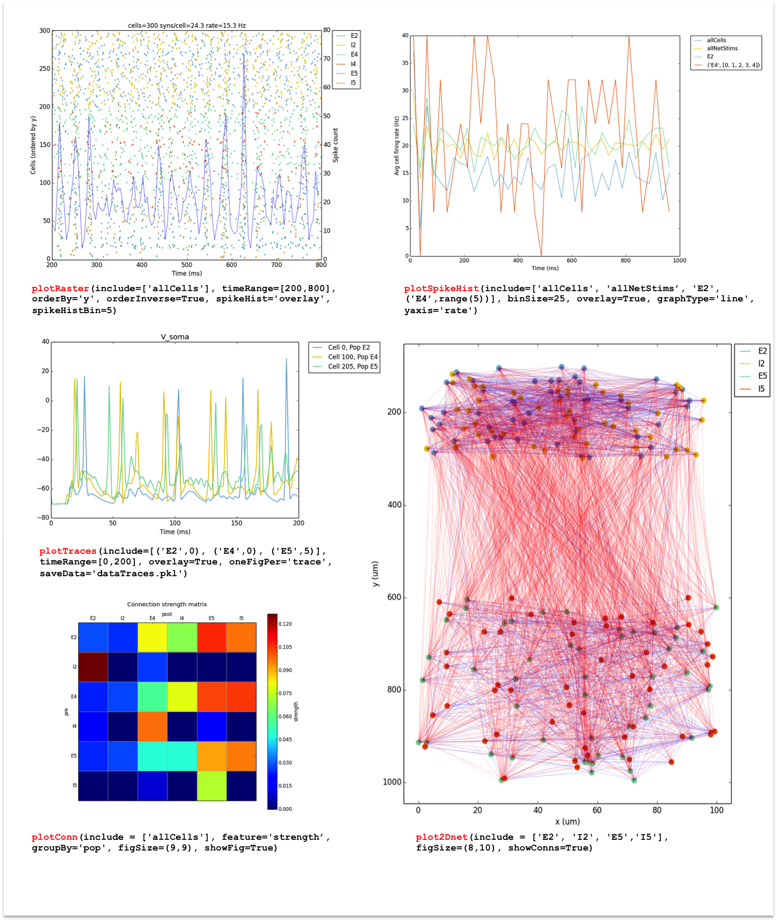
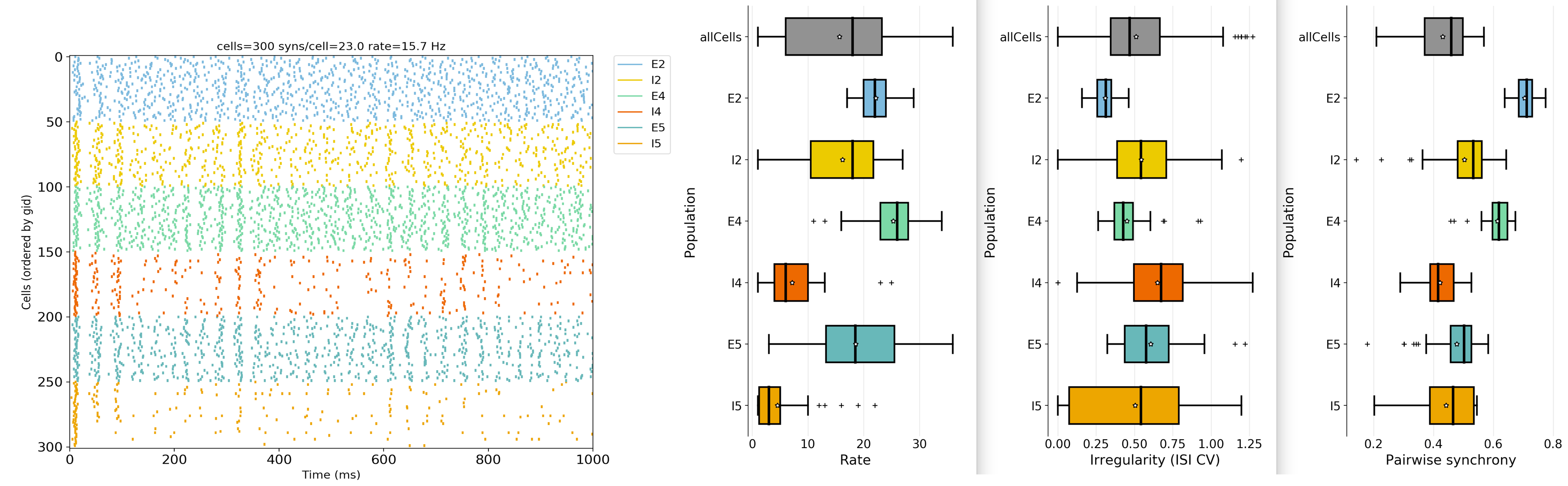
Network class methods
Methods to set up network
net.setParams()
net.createPops()
net.createCells()
net.connectCells()
Methods to modify network
net.modifyCells(params, updateMasterAllCells=False)
Modifies properties of cells in an instantiated network. The
paramsargument is a dictionary with the following item:‘secs’: dictionary of sections using same format as for initial setting of cell property rules (see Cell types or Cell class for details)
e.g.
{'soma': {'geom': {'L': 100}}}sets the soma length to 100 um.
net.modifySynMechs(params, updateMasterAllCells=False)
Modifies properties of synMechs in an instantiated network. The
paramsargument is a dictionary with the following 3 items:‘conds’: dictionary of conditions to select synMechs that will be modified, with each item containing a synMech tag, and the desired value ([min, max] range format allowed).
e.g.
{'label': 'AMPA', 'sec': 'soma', 'loc': [0, 0.5]}targets synMechs with the label ‘AMPA’, at the soma section, with locations between 0 and 0.5.‘cellConds’: dictionary of conditions to select target cells that will contain the synMechs to be modified, with each item containing a cell tag (see list of tags available Cell class), and the desired value ([min, max] range format allowed).
e.g.
{'pop': 'PYR', 'ynorm': [0.1, 0.6]}targets connections of cells from the ‘PYR’ population with normalized depth within 0.1 and 0.6.‘[synMech property]’ (e.g. ‘tau1’ or ‘e’): New value for stim property (note that properties depend on the type of synMech). Can include several synMech properties to modify.
net.modifyConns(params, updateMasterAllCells=False)
Modifies properties of connections in an instantiated network. The
paramsargument is a dictionary with the following 3 items:‘conds’: dictionary of conditions to select connections that will be modified, with each item containing a conn tag (see list of conn tags available Cell class), and the desired value ([min, max] range format allowed).
e.g.
{'label': 'M->S'}targets connections that were created using the connParams rule labeled ‘M->S’. e.g.{'weight': [0.4, 0.8], 'sec': 'soma'}targets connections with weight within 0.4 and 0.8, and that were made onto the ‘soma’ section.‘postConds’: dictionary of conditions to select postsynaptic cells that will contain the connections to be modified, with each item containing a cell tag (see list of tags available Cell class), and the desired value ([min, max] range format allowed).
e.g.
{'pop': 'PYR', 'ynorm': [0.1, 0.6]}targets connections of cells from the ‘PYR’ population with normalized depth within 0.1 and 0.6.‘weight’ | ‘threshold’: New value for connection weight or threshold. Can include both.
net.modifyStims(params, updateMasterAllCells=False)
Modifies properties of stim in an instantiated network. The
paramsargument is a dictionary with the following 3 items:‘conds’: dictionary of conditions to select stims that will be modified, with each item containing a stim tag (see list of stim tags available Cell class), and the desired value ([min, max] range format allowed).
e.g.
{'label': 'VClamp1->S'}targets stims that were created using the stimTargetParms rule labeled ‘VClamp1->S’. e.g.{'source': 'IClamp2', 'dur': [100, 300]}targets stims that have as source ‘Netstim2’ (defined in stimSourceParams), with a duration between 100 and 300 ms.‘cellConds’: dictionary of conditions to select target cells that will contain the stims to be modified, with each item containing a cell tag (see list of tags available Cell class), and the desired value ([min, max] range format allowed).
e.g.
{'pop': 'PYR', 'ynorm': [0.1, 0.6]}targets connections of cells from the ‘PYR’ population with normalized depth within 0.1 and 0.6.‘[stim property]’ (e.g. ‘dur’, ‘amp’ or ‘delay’): New value for stim property (note that properties depend on the type of stim). Can include several stim properties to modify.
Note
The updateMasterAllCells argument ensures that the sim.net.allCells list in the master node is also updated with the modified parameters. By default this is set to False, since it slows down the modify functions, and sim.net.allCells will be updated automatically after running simulation and gathering data.
Population class methods
pop.createCells()
pop.createCellsFixedNum()
pop.createCellsDensity()
pop.createCellsList()
Cell class methods
cell.create()
cell.createPyStruct()
cell.createNEURONObj()
cell.associateGid()
cell.addConn()
cell.addNetStim()
cell.addIClamp()
cell.recordTraces()
cell.recordStimSpikes()
NetPyNE data model (structure of instantiated network and output data)
A representation of the instantiated network structure generated by NetPyNE is shown below:
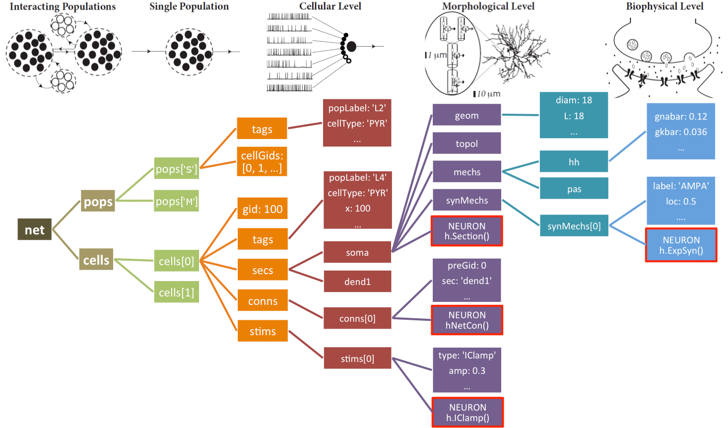
NetPyNE data model: Structure of instantiated network
The model is instantiated in sim.net as a Network object. This object has a number of intrisic attributes, and others may or may not be present depending on particular implementations. The two basic elements composing “sim.net” are:
pops - An ordered dictionary describing all populations implemented in the network. Its entries are a key labeling the population (as defined in
netParams.popParams) and a value referencing the Pop object. This object has a number of attributes:tags: Dictionary describing different attributes of the population, related to the declaration rule that defines it. For example:
sim.net.pops['Exc_L4'].tags = {'cellType': 'PYR', 'numCells': 100, 'pop': 'Exc_L4'}cellGids: List of neuron identifiers (global ids) composing the population. For example:
sim.net.pops['Exc_L4'].cellGids = [0, 1, 2, 3, 4]cellModelClass: Type describing which particular cell model class was implemented (e.g.
compartCellorpointCell).
cells - A list of cells instantiated locally (this disctinction is important when implementing parallel computing). Each element in the list is a Cell object (among different cell model classes). As a Cell object, there are a number of intrinsic attributes:
gid: cell global identification number
tags: Dictionary describing different attributes of the cell, which may include some tags from the population it belongs to (tags list in
netParams.popTagsCopiedToCells, for example ‘cellType’). These attributes are:pop: Label of the population it belongs to. For example:
sim.net.cells[0].tags['pop'] = 'Exc_L4'x, y, z: Cell’s x-, y-, z-coordinates. For example:
sim.net.cells[0].tags['x'] = -2.3535xnorm, ynorm, znorm: Cell’s x-, y-, z-normalized coordinates.
Other tags depending on particular situations (for example, declaring populations in
netParams.popParamswith acellsList, includingparams).
conns: List of connections (this cell at the post-synaptic side). Each element in this list (a particular connection) is a dictionary with the following entries:
preGid: Identity of the presynaptic cell (Gid). In the case this connection arises from a stimulation that requires a connection, the value will correspond to ‘NetStim’.
weight: Weight of the connection.
delay: Delay of the connection.
synMech: Label of the synaptic mechanism governing this connection.
Depending on different scenarios, other entries will appear:
- If the cell model class is NOT a point process, there will be a section/location where the synapse is put on. Then, these entries will appear:
sec: Section hosting the synapse.
loc: Location within this section where the synapse is displayed.
If the connection is specified as a gap junction (
netParams.connParams['rule']['gapJunction']= True, only available for ‘compartCell’ cell model class), entries associated to this kind of connections will appear:gapJunction: Connection side (‘pre’ or ‘post’), as specified by the rule.
preLoc: Gap junction location at pre-synaptic side, as specified by the rule (for cells at ‘post’).
gapId: Id of the cell at its connection side.
preGapId: Id of the cell at other connection side.
shape, plast, weightIndex: Entries used for implementing specific connectivity patterns or processes.
hObj: Except for the case of gap junctions, all other connections are implemented via NEURON
NetConobjects. The object itself is the value correspoding to this ‘hObj’ key. So, the NEURON object can be accessed (and modified) with, for example,sim.net.cells[0].conns[0]['hObj']
In particular, methods corresponding to these objects can be called from command line (once the network has been instantiated). For example:
sim.net.cells[0].conns[0]['hObj'].syn().stims: List of stimuli incoming to the cell. Each element in this list is a dictionary with the following entries:
label: Label of the rule specifying target parameters
source: Label of the source rule that defines the incoming stimulus.
type: Type of stimulus. For example:
sim.net.cells[0].stims[0]['type'] = 'NetStim'orsim.net.cells[0].stims[0]['type'] = 'IClamp'sec: Section where the stimulus is targeting.
loc: Location within the section where the stimulus is impinging on.
Properties defining the incoming stimuli. For example, ‘rate’, ‘noise’, ‘start’, and ‘number’ for NetStim (plus ‘seed’ to initialize the random generator).
hObj: NEURON object associated to the stimuli. For example:
sim.net.cells[0].stims[0]['hObj']
Methods associated to the NEURON object are readily available. For example, if the object is an ‘IClamp’, then we can change its duration via
sim.net.cells[0].stims[0]['hObj'].durDepending on the cell model class, other entries are available. In particular, for the ‘compartCell’ cell model class, the following one:
secs: Dictionary with the sections composing the cell. Within this dictionary, the following entries:
geom: Dictionary with the geometrical properties of the cylinder composing the section. For example,
sim.net.cells[0].secs['soma']['geom'] = {diam: 18.8, L: 18.8, Ra: 123.0}topol: Dictionary with the specifications of the topology (how is it connected to other sections).
mechs: Dictionary with distributed mechanisms. For example,
sim.net.cells[0].secs['soma']['mechs']['hh'] = {gnabar: 0.12, gkbar: 0.036, gl: 0.003, el: -70}ions: Dictionary specyfing ionic mechanisms included in the section.
synMechs: List of all synapses located at this section. Each element in this list is a dictionary with all the information related to it:
label: Label describing the rule that specifies the synaptic dynamics.
loc: Location within the section where the synapse is displayed
properties associated to the definition of the synaptic model. For example, ‘tau1’, ‘e’, etcetera.
hObj: NEURON object associated to the synapse. For example
sim.net.cells[0].secs['soma']['synMechs'][0]['hObj'] = Exp2Syn[0]
pointps: Dictionary specifying a point process governing the voltage dynamics of the section, including the name of the ‘mod’ where the nonlinear mechanism is defined and all neccessary parameters.
Other scalar properties: spikeGenLoc, vinit, etcetera.
hObj: NEURON object associated to the section. For example,
type(sim.net.cells[0].secs['soma']['hObj']) = nrn.Section
Beyond these two elements (‘pops’ and ‘cells’), there are a number of elements also defining and composing “sim.net”:
allPops: Dictionary with all populations composing the network. Each key correspond to a defined population, and its value is a dictionary with information about it (‘tags’, ‘cellGids’, etc).
allCells: List with information about all cells (global). Each element/cell is a dictionary with all the information defining this cell.
params: netParams specifying the network.
rxd: Dictionary with all the specifications of a Reaction-Diffusion model (same format as in
netParams.rxdParams) PLUS the associated NEURON objects.recXElectrode: Object associated to recording LFP (if any).
compartCells and popForEachGid: Object cells and a dictionary, {‘gid’: ‘pop’}, for use during LFP and dipole recording.
cells_dpls and cells_dpl: Dictionary with vectors of dipoles for each cell, over time and at one time, for use during LFP and dipole recording.
gid2lid: Dictionary mapping global to local ids, {‘gid’: ‘lid’}.
lastGid: Last cell’s Gid defined. Useful during development of the network.
lastGapId: Last gap junction defined. Useful during development of the network.
preGapJunctions: List storing information about presynaptic side, according to the direction written in the connectivity rule, for gap junctions.
Accessing dictionaries using dot notation: Dict and ODict classes
In order to allow dot notation (a.b.c) to access NetPyNE structures we have added the Dict an ODict classes which are subclasses that inherit from the original Python dict and OrderedDict classes. All NetPyNE internal dictionaries are either of class Dict or ODict. Below are some features of the Dict class:
Can be accessed either using standard dict methods:
a['b']['c'],a.iteritems(),a.keys(),a.update(), etc.), or attribute methods / dot notation:a.b.c=2.Missing elements are automatically added (note this can have undesired effects if you use the wrong keys):
a=Dict(); a.b.c.d.e=1The constructor allows a dict (including nested dicts) and/or kwargs:
a=Dict(b=1, c=2)or ``a=Dict({‘a’: 1, ‘b’: {‘c’: 2}})`The method .todict() returns the dict version of Dict:
a=Dict({'b':1}); a_dict=a.todict()Serialization via __getstate__() method (eg. when pickled) returns a normal dict (using .todict() method).
To specify the netParams you can use either standard dicts or the Dict() class. To use the Dict class you first need to import it via:
from netpyne.specs import Dict
Examples of accessing NetPyNE structures via dot notation:
cellRule = Dict(); cellParam.secs.soma.mechs.hh = {'gnabar': 0.12, 'gkbar': 0.036}; cellParam.conds = {'cellType': 'IT'}
netParams.cellParams.PYR_rule.secs.soma.mechs.hh.gnabar
simConfig.analysis.plotRaster.include = ['all']
sim.net.cells[0].secs.soma.mechs.nap.gbar = 0.1
sim.net.cells[0].secs.soma.hSec(0.5).gbar_nap = 0.1
sim.net.allCells[5].tags.pop
sim.net.cells[0].conns[1].weight
sim.net.cells[0].conns[1].hNetcon.weight[0]
sim.net.cells[0].stims[0].type
sim.net.pops.PYRpop.tags
sim.net.allPops.Mpop.cellGids
sim.allSimData.spkt
sim.allSimData.stims.cell_31.Input_4
sim.allSimData.V_soma.cell_1
Sim module
net (Network object)
cfg (SimConfig object)
pc (h.ParallelContext object)
nhosts (int)
rank (int)
timingData (Dict)
Network class
pops (Dict of Pop objects)
cells (list of Cell objects)
params (NetParams object)
After gathering from nodes: - allCells (list of Dicts) - allPops (list of Dicts)
Population class
cellGids (list)
tags (Dict)
Cell class
gid (int)
- tags (Dict)
‘label’
‘pop’
‘cellModel’
‘cellType’
‘x’, ‘y’, ‘z’
‘xnorm’, ‘ynorm’, ‘znorm’
- secs (Dict)
- ‘secName’ (e.g. ‘soma’) (Dict)
‘hSec’ (NEURON object)
- ‘geom’ (Dict)
‘L’
‘diam’
‘pt3d’ (list of tuples)
…
- ‘topol’ (Dict)
‘parentSec’
‘parentX’
‘childX’
- ‘mechs’ (Dict)
- ‘mechName’ (e.g. ‘hh’) (Dict)
‘gnabar’
‘gkbar’
…
- ‘pointps’ (Dict)
- ‘pointpName’ (e.g. ‘Izhi’) (Dict)
‘hPointp’ (NEURON object)
‘mod’
‘a’
‘b’
…
- ‘synMechs’ (list)
- [0] (Dict)
‘hObj’: NEURON object
‘label’
‘loc’
- secLists (Dict)
‘secListName’ (e.g. ‘alldends’) (list)
- conns (list)
- [0] (Dict)
‘hNetCon’: NEURON object
‘label’
‘preGid’
‘preLabel’
‘sec’
‘loc’
‘synMech’
‘weight’
‘threshold’
- stims (list)
- [0] (Dict)
‘hIClamp’ (NEURON object)
‘source’
‘type’
‘label’
‘sec’
‘loc’
‘amp’
‘dur’
‘delay’
Simulation output data
The output data of simulation is stored in dictionaries sim.simData and sim.allSimData. The former should be used in sinlge process environment, while the latter contains data gathered from all nodes from parallel context.
The contents of simulation output data depend on the settings in simConfig, and may contain the following.
1. Traces of cells
Keys of simData correspond to keys of simConfig.recordTraces (e.g. ‘V_soma’), with the value of each trace containing in turn a dictionary with the list of cells for which this traces was recorded. The recorded traces will be stored as h.Vector for each cell. For example, for simConfig setting:
simConfig.recordTraces = {'V_soma':{'sec':'soma','loc':0.5,'var':'v'},
                          'Ina_soma':{'sec':'soma','loc':0.5,'var':'ina'}}
simConfig.recordCells = [1, 3]
simConfig.recordStep = 0.1
the simData dictionary will contain (among others):
{'V_soma': {'cell_1': <h.Vector>, 'cell_3': <h.Vector>},
 'Ina_soma': {'cell_1': <h.Vector>, 'cell_3': <h.Vector>}
where the length of each Vector depends on simConfig.duration and simConfig.recordStep
2. Spikes
spkt, spkid - ordered lists of spike times and cell gids for each spike.
The simConfig.recordCellsSpikes (True, by default) can be used to record only from a subset of cells or turn off spike recordig.
3. Stimuli to the network
stims. For each population of NetStim or VecStim it contains the list of spike times (h.Vector) for each target cell.
Only available if simConfig.recordStim is True.
4. LFP-related data
LFP, LFPCells, LFPPops. Depend on the recordLFP, saveLFPCells, saveLFPPops options in simConfig.
LFP- is an np.array of LFP values of shape(num timesteps, num electrodes)LFPCells- dictionary of LFP data recorded from each cell (LFP data is in format as above)LFPPops- dictionary of average LFP data recorded from each population (LFP data is in format as above)iMembrane- dictionary of transmembrane current of each cell. An np.array of shape(num timesteps, num segments), where num segments is the total number of segments accross all sections of the cell.
5. Dipole-related data
dipoleSum, dipoleCells, dipolePops. Depend on the recordDipole, saveDipoleCells, saveDipolePops options in simConfig
dipoleSum- sum of current dipole moments at each timestep(num timesteps, 3); can be used for EEG/MEG calculationdipoleCells- dictionary of current dipole moments recorded for each cell (dipoles data is in format as above)dipolePops- dictionary of average current dipole moments recorded for each population (dipoles data is in format as above)
Data saved to file
simConfig
netParams
net
simData
Importing externally-defined cell models
NetPyNE provides support for internally defining cell properties of for example Hodgkin-Huxley type cells with one or multiple compartments, or Izhikevich type cells (eg. see NetPyNE Tutorial). However, it is also possible to import previously defined cells in external files eg. in hoc cell templates, or cell classes, using the importCellParams() method. This method will convert all the cell information into the required NetPyNE format. This way it is possible to make use of cells which have been implemented separately.
The cellRule = netParams.importCellParams(label, conds, fileName, cellName, cellArgs={}, importSynMechs=False) method takes as arguments the label of the new cell rule, the name of the file where the cell is defined (either .py or .hoc files), and the name of the cell template (hoc) or class (python). Optionally, a set of arguments can be passed to the cell template/class (eg. {'type': 'RS'}). If you wish to import the synaptic mechanisms parameters, you can set the importSynMechs=True. The method returns the new cell rule so that it can be further modified.
NetPyNE contains NO built-in information about any of the cell models being imported. Importing is based on temporarily instantiating the external cell model and reading all the required information (geometry, topology, distributed mechanisms, point processes, etc.).
Below we show example of importing 10 different cell models from external files. For each one we provide the required files as well as the NetPyNE code. Make sure you run nrnivmodl to compile the mod files for each example. The list of example cell models is:
Additionally, we provide an example NetPyNE file (tut_import.py) which imports all 10 cell models, creates a population of each type, provides background inputs, and randomly connects all cells. To run the example you also need to download all the files where cells models are defined and the mod files (see below). The resulting raster is shown below:
Hodgkin-Huxley model
Description: A 2-compartment (soma and dendrite) cell with hh and pas mechanisms, and synaptic mechanisms. Defined as a Python class.
Required files:
HHCellFile.py
NetPyNE Code
netParams.importCellParams(
        label='PYR_HH_rule',
        conds={'cellType': 'PYR', 'cellModel': 'HH'},
        fileName='HHCellFile.py',
        cellName='HHCellClass',
        importSynMechs=True)
Hodgkin-Huxley model with 3D geometry (from .hoc)
Description: A multi-compartment cell. Defined as a HOC cell template. Only the cell geometry is included. Example of importing only geometry, and then adding biophysics (hh and pas channels) from NetPyNE.
Required files:
geom.hoc
NetPyNE Code:
cellRule = netParams.importCellParams(
        label='PYR_HH3D_hoc',
        conds={'cellType': 'PYR', 'cellModel': 'HH3D'},
        fileName='geom.hoc',
        cellName='E21',
        importSynMechs=False)

cellRule['secs']['soma']['mechs']['hh'] = {'gnabar': 0.12, 'gkbar': 0.036, 'gl': 0.003, 'el': -70} # soma hh mechanism

for secName in cellRule['secs']:
        cellRule['secs'][secName]['mechs']['pas'] = {'g': 0.0000357, 'e': -70}
        cellRule['secs'][secName]['geom']['cm'] = 1
Hodgkin-Huxley model with 3D geometry (from .swc)
Description: A multi-compartment cell, with imported morphology from an SWC file. Only the cell geometry is included. Example of importing only geometry, and then adding biophysics (hh and pas channels) from NetPyNE.
Importing a morphology into NetPyNE from an SWC file is simple, but NetPyNE does no testing or validation of morphologies, so you should ensure your morphology file is accurate and valid before using it in NetPyNE.
Required files:
BS0284.swc
NetPyNE Code:
cellRule = netParams.importCellParams(
        label='PYR_HH3D_swc',
        conds={'cellType': 'PYR', 'cellModel': 'HH3D'},
        fileName='BS0284.swc',
        cellName='swc_cell')

netParams.renameCellParamsSec('PYR_HH3D_swc_rule', 'soma_0', 'soma')  # rename imported section 'soma_0' to 'soma'

for secName in cellRule['secs']:
        cellRule['secs'][secName]['mechs']['pas'] = {'g': 0.0000357, 'e': -70}
        cellRule['secs'][secName]['geom']['cm'] = 1
        if secName.startswith('soma'):
                cellRule['secs'][secName]['mechs']['hh'] = {'gnabar': 0.12, 'gkbar': 0.036, 'gl': 0.003, 'el': -70}
Traub model
Description: Traub cell model defined as hoc cell template. Requires multiple mechanisms defined in mod files. Downloaded from ModelDB and modified to remove calls to figure plotting and others. The km mechanism was renamed km2 to avoid collision with a different km mechanism required for the Traub cell model. Synapse added from NetPyNE.
ModelDB link: http://senselab.med.yale.edu/ModelDB/showmodel.cshtml?model=20756
Required files:
pyr3_traub.hoc,
ar.mod,
cad.mod,
cal.mod,
cat.mod,
k2.mod,
ka.mod,
kahp.mod,
kc.mod,
kdr.mod,
km2.mod,
naf.mod,
nap.mod
NetPyNE Code:
cellRule = netParams.importCellParams(
        label='PYR_Traub_rule',
        conds= {'cellType': 'PYR', 'cellModel': 'Traub'},
        fileName='pyr3_traub.hoc',
        cellName='pyr3')

somaSec = cellRule['secLists']['Soma'][0]

cellRule['secs'][somaSec]['spikeGenLoc'] = 0.5
Mainen model
Description: Mainen cell model defined as python class. Requires multiple mechanisms defined in mod files. Adapted to python from hoc ModelDB version. Synapse added from NetPyNE.
ModelDB link: http://senselab.med.yale.edu/ModelDB/showModel.cshtml?model=2488 (old hoc version)
Required files:
mainen.py,
cadad.mod,
kca.mod,
km.mod,
kv.mod,
naz.mod,
Nca.mod
NetPyNE Code:
netParams.importCellParams(
        label='PYR_Mainen_rule',
        conds={'cellType': 'PYR', 'cellModel': 'Mainen'},
        fileName='mainen.py',
        cellName='PYR2')
Friesen model
Required files: Friesen cell model defined as python class. Requires multiple mechanisms (including point processes) defined in mod files. Spike generation happens at the axon section (not the soma). This is indicated in NetPyNE adding the spikeGenLoc item to the axon section entry, and specifying the section location (eg. 0.5).
Required files:
friesen.py,
A.mod,
GABAa.mod,
AMPA.mod,
NMDA.mod,
OFThpo.mod,
OFThresh.mod,
netcon.inc,
ofc.inc
NetPyNE Code:
cellRule = netParams.importCellParams(
        label='PYR_Friesen_rule',
        conds={'cellType': 'PYR', 'cellModel': 'Friesen'},
        fileName='friesen.py',
        cellName='MakeRSFCELL')

cellRule['secs']['axon']['spikeGenLoc'] = 0.5  # spike generator location.
Izhikevich 2003a model (independent voltage variable)
Description: Izhikevich, 2003 cell model defined as python class. Requires point process defined in mod file. This version is added to a section but does not employ the section voltage or synaptic mechanisms. Instead it uses its own internal voltage variable and synaptic mechanism. This is indicated in NetPyNE adding the vref item to the point process entry, and specifying the name of the internal voltage variable (V).
Modeldb link: https://senselab.med.yale.edu/modeldb/showModel.cshtml?model=39948
Required files:
izhi2003Wrapper.py,
izhi2003a.mod
NetPyNE Code:
cellRule = netParams.importCellParams(
        label='PYR_Izhi03a_rule',
        conds={'cellType': 'PYR', 'cellModel':'Izhi2003a'},
        fileName='izhi2003Wrapper.py',
        cellName='IzhiCell',
        cellArgs={'type':'tonic spiking', 'host':'dummy'})

cellRule['secs']['soma']['pointps']['Izhi2003a_0']['vref'] = 'V' # specify that uses its own voltage V
Izhikevich 2003b model (uses section voltage)
Description: Izhikevich, 2003 cell model defined as python class. Requires point process defined in mod file. This version is added to a section and shares the section voltage and synaptic mechanisms. A synaptic mechanism is added from NetPyNE during the connection phase.
Modeldb link: https://senselab.med.yale.edu/modeldb/showModel.cshtml?model=39948
Required files:
izhi2003Wrapper.py,
izhi2003b.mod
NetPyNE Code:
netParams.importCellParams(
        label='PYR_Izhi03b_rule',
        conds={'cellType': 'PYR', 'cellModel':'Izhi2003b'},
        fileName='izhi2003Wrapper.py',
        cellName='IzhiCell',
        cellArgs={'type':'tonic spiking'})
Izhikevich 2007a model (independent voltage variable)
Description: Izhikevich, 2007 cell model defined as python clas. Requires point process defined in mod file. This version is added to a section but does not employ the section voltage or synaptic mechanisms. Instead it uses its own internal voltage variable and synaptic mechanism. This is indicated in NetPyNE adding the vref item to the point process entry, and specifying the name of the internal voltage variable (V). The cell model includes several internal synaptic mechanisms, which can be specified as a list in NetPyNE by adding the synList item to the point process entry.
Modeldb link: https://senselab.med.yale.edu/modeldb/showModel.cshtml?model=39948
Required files:
izhi2007Wrapper.py,
izhi2007a.mod
NetPyNE Code:
cellRule = netParams.importCellParams(
        label='PYR_Izhi07a_rule',
        conds={'cellType': 'PYR', 'cellModel':'Izhi2007a'},
        fileName='izhi2007Wrapper.py',
        cellName='IzhiCell',
        cellArgs={'type':'RS', 'host':'dummy'})

cellRule['secs']['soma']['pointps']['Izhi2007a_0']['vref'] = 'V' # specify that uses its own voltage V

cellRule['secs']['soma']['pointps']['Izhi2007a_0']['synList'] = ['AMPA', 'NMDA', 'GABAA', 'GABAB']  # specify its own synapses
Izhikevich 2007b model (uses section voltage)
Description: Izhikevich, 2007 cell model defined as python class. Requires point process defined in mod file. This version is added to a section and shares the section voltage and synaptic mechanisms.
Modeldb link: https://senselab.med.yale.edu/modeldb/showModel.cshtml?model=39948
Required files:
izhi2007Wrapper.py,
izhi2007b.mod
NetPyNE Code:
netParams.importCellParams(
        label='PYR_Izhi07b_rule',
        conds={'cellType': 'PYR', 'cellModel':'Izhi2007b'},
        fileName='izhi2007Wrapper.py',
        cellName='IzhiCell',
        cellArgs={'type':'RS'})
The full code to import all cell models above and create a network with them is available here: tut_import.py.
Parameter Optimization of a Simple Neural Network Using An Evolutionary Algorithm
This tutorial provides an example of how to use inspyred, an evolutionary algorithm toolkit, to optimize parameters in our prior tut2.py** neural network–modified to remove any code relating to initiating network simulation and output display–, such that it achieves a target average firing rate around (~) 17 Hz.
**Some modification is required near the end of the tut2.py code, to
remove any code relating to initiating network simulation and output
display, all of which has now been handled in the new top level code
(tut_optimization.py):
# Create network and run simulation
# sim.createSimulateAnalyze(netParams = netParams, simConfig = simConfig)   # line commented out

# import pylab; pylab.show()  # if figures appear empty   # line commented out
excerpt from tut2.py
Additional Background Reading
A description of the algorithm methodology that will be used to optimize the simple neural network in this example.
Introduction
Using the inspyred python package to find neural network parameters so that some property of the network (e.g. firing rate) matches a desired target can be broken down into 3 steps. First, 1) defining a desired target model (in this case, some measurable value) and fitness function–fitness defined here as a calculable value that represents how close a neural network with a given parameters matches the target. Subsequently, it is necessary to 2) determine the appropriate neural network parameters to modify to achieve that model/value. Finally, 3) appropriate parameters for the evolutionary algorithm are defined. Ultimately, If the inputs to the evolutionary algorithm are appropriate, then over successive iterations, the parameters determined by the evolutionary algorithm should generate models closer to the target.
Particularizing these 3 steps to our example we get:
Defining a desired target model and fitness function.
Defining a desired target model is largely arbitrary, some constraints being that there must be a way to adjust parameters such that the results are closer to the target model than before (or that fitness is improved), and that there must be a way to evaluate the fitness of a model with given parameters. In this case, our target model is a neural network that achieves an average firing rate of 17 Hz. The fitness for such a model can be defined as the difference between the average firing rate of a certain model and the target firing rate of 17 Hz.
Selecting the model parameters to be optimized.
If a parameter can in some way alter the fitness of the final model, it may be an appropriate candidate for optimization, depending on what the model is seeking to achieve. As well as a host of other parameters, altering the probability, weight or delay of the synaptic connections in the neural network can affect the average firing rate. In this example, we will optimize the values of the probability, weight and delay of connections from the sensory to the motor population.
Selecting appropriate parameters for the evolutionary algorithm.
inspyred allows customization of the various components of the evolutionary algorithm, including:
a selector that determines which sets of parameter values become parents and thus which parameter values will be used to form the next generation in the evolutionary iteration,
a variator that determines how each current iteration of parameter sets is formed from the previous iteration,
a replacer which determines whether previous sets of parameter values are brought into the next iteration,
a terminator which defines when to end evolutionary iterations,
an observer which allows for tracking of parameter values through each evolutionary iteration.
Using inspyred
The evolutionary algorithm is implemented the ec module from the inspyred package:
from inspyred import ec # import evolutionary computation from inspyred
excerpt from tut_optimization.py
ec includes a class for the evolutionary computation algorithm: ec.EvolutionaryComputation(), which allows entering parameters to customize the algorithm. The evolutionary algorithm involves random processes (e.g. randomly mutating genes) and so requires random number generator. In this case we will use python’s Random() method, which we initialize using a specific seed value so that we can reproduce the results in the future:
# create random seed for evolutionary computation algorithm
rand = Random()
rand.seed(1)

# instantiate evolutionary computation algorithm
my_ec = ec.EvolutionaryComputation(rand)
excerpt from tut_optimization.py
Parameters for the evolutionary algorithm are then established for our ec evolutionary computation instance by assigning various variator, replacer, terminator and observer elements–essentially toggling specific components of the algorithm– to ec.selectors, ec.variators, ec.replacers, ec.terminators, ec.observers:
#toggle variators
my_ec.variator = [ec.variators.uniform_crossover, # implement uniform crossover & gaussian replacement
                ec.variators.gaussian_mutation]
my_ec.replacer = ec.replacers.generational_replacement   # implement generational replacement

my_ec.terminator = ec.terminators.evaluation_termination # termination dictated by no. evaluations

#toggle observers
my_ec.observer = [ec.observers.stats_observer,  # print evolutionary computation statistics
                ec.observers.plot_observer,   # plot output of the evolutionary computation as graph
                ec.observers.best_observer]   # print the best individual in the population to screen
excerpt from ex_optimization.py
where:
ec.variators.uniform_crossover |
variator where coin flip to determine whether ‘mom’ or ‘dad’ element is inherited by offspring |
ec.variators.gaussian_mutation |
variator implements gaussian mutation which makes use of bounder function as specified in: my_ec.evolve(…,bounder=ec.Bou nder(minParamValues, maxParamValues) ,…) |
ec.replacers.generational_replacement |
replacer implements generational replacement with elitism (as specified in my_ec.evolve(…,num_elites=1,…) , where the existing generation is replaced by offspring, and <num_elites> existing individuals will survive if they have better fitness than the offspring |
ec.terminators.evaluation_termination |
terminator runs based on the number of evaluations that have occurred |
ec.observers.stats_observer |
indicates how many of the generated individuals (parameter sets) will be selected for the next evolutionary iteration. |
ec.observers.plot_observer |
indicates the rate of mutation, or the rate at which values for each parameter (probability, weight and delay) taken from a prior generation are altered in the next generation |
ec.observers.best_observer |
sets the number of parameters that will be optimized to 3, corresponding to the length of [probability, weight, delay]. |
These predefined selector, variator, replacer, terminator and observer elements as well as other options can be found in the inspyred documentation.
FInally, the evolutionary computation algorithm instance includes a method: my_ec.evolve() , which will move through successive evolutionary iterations evaluating different parameter sets until the terminating condition is achieved. This function comes with multiple arguments, with two significant arguments being the generator and evaluator functions. A function call for my_ec.evolve() will look similar to the following:
# call evolution iterator

final_pop = my_ec.evolve(generator=generate_netparams, # assign model parameter generator to iterator generator
                      evaluator=evaluate_netparams, # assign fitness function to iterator evaluator
                      pop_size=10,
                      maximize=False,
                      bounder=ec.Bounder(minParamValues, maxParamValues),
                      max_evaluations=50,
                      num_selected=10,
                      mutation_rate=0.2,
                      num_inputs=3,
                      num_elites=1)
excerpt from tut_optimization.py
where:
pop_size=10 |
means that each generation of parameter sets will consist of 10 individuals |
maximize=False |
means that we are taking higher fitness to correspond to minimal values in terms of difference between model firing frequency and 17 Hz |
|
defines boundaries for each of the parameters. The format to describe the minimum and maximum values for the parameters we are seeking to optimize: minParamValues is an array of minimum of values corresponding to [probability, weight, delay], and maxParamValues is the array of maximum values. |
max_evaluations=50 |
indicates how many parameter sets are evaluated prior termination of the evolutionary iterations |
num_selected=10 |
indicates how many of the generated individuals (parameter sets) will be selected for the next evolutionary iteration. |
mutation_rate=0.2 |
indicates the rate of mutation, or the rate at which values for each parameter (probability, weight and delay) taken from a prior generation are altered in the next generation |
num_inputs=3 |
sets the number of parameters that will be optimized to 3, corresponding to the length of [probability, weight, delay]. |
num_elites=1 |
sets the number of elites to 1. That is, one individual from the existing generation may be retained (as opposed to a complete generational replacement) if it has better fitness than an individual selected from the offspring. |
The generator and evaluator arguments expect user defined functions as inputs, with generator used to define a population of initial parameter value sets for the very first iteration, and evaluator being the fitness function that will be used to evaluate each model for how close it is to the target. In this example, the generator is a fairly straightforward function which creates an initial set of parameter values (i.e. [probability, weight, delay] ) by drawing from a parameterized uniform distribution:
# return a set of initialParams which contains a [probability, weight, delay]

def generate_netparams(random, args):

    size = args.get('num_inputs')
    initialParams = [random.uniform(minParamValues[i], maxParamValues[i]) for i in range(size)]

return initialParams
excerpt from tut_optimization.py
The fitness function involves taking a list of sets of parameter values, i.e. : [ [ a0, b0, c0], [a1, b1, c1], [a2, b2, c2], … , [an, bn, cn ] ] where a, b, c represent the parameter values and 1 through n representing the individual number within the population, and calculating a fitness score for each element of the list, which is then returned as a list of fitness values (i.e. : [ f0, f1, f2, … , fn ] ) corresponding to the initial sets of parameter values. It follows the general template:
def evaluate_fitness(candidates, args):
   fitness = []
   for candidate in candidates:
       fit = some_fitness_function(candidate)
       fitness.append(fit)
   return fitness
excerpt from tut_optimization.py
The actual code that is used to serve as some_fitness_function(candidate) is described below:
Overview of the Fitness Function
The fitness function in this case involves 1) creating a neural network with the given parameters, 2) simulating it to find the average firing rate, then 3) comparing this firing rate to a target firing rate.
Creating a neural network with the parameters to evaluate
We will employ the NetPyNE defined network in tut2.py, and modify the [probability, weight, delay] parameters. This involves redefining specific values found in tut2.py found within the connectivity rule between the S and M populations: netParams.connParams[‘S->M’]
## Cell connectivity rules
netParams.connParams['S->M'] = {      #  S -> M label
      'preConds': {'popLabel': 'S'},  # conditions of presyn cells
      'postConds': {'popLabel': 'M'}, # conditions of postsyn cells
      'probability': 0.5,             # probability of connection <-- to be optimized by evolutionary algorithm
      'weight': 0.01,                 # synaptic weight           <-- to be optimized by evolutionary algorithm
      'delay': 5,                     # transmission delay (ms)   <-- to be optimized by evolutionary algorithm
      'synMech': 'exc'}               # synaptic mechanism
excerpt from tut2.py
these values are replaced in the fitness function with the parameter values generated by the evolutionary algorithm. As the fitness function resides within a for loop iterating through the list of candidates ( for icand,cand in enumerate(candidates): ), the individual parameters can be accessed as cand[0], cand[1], and cand[2]. Reassigning values to the parameters in tut_optimization.py can be done via the following line:
tut2.netParams.connParams['S->M']['<parameter>'] = <value>
Simulating the created neural network and finding the average firing rate
Once the network parameters have been modified we can call the sim.createSimulate() NetPyNE function to run the simulation. We will pass as arguments the tut2 netParams and simConfig objects that we just modified. Once the simulation has ran we will have access to the simulation output via sim.simData.
# create network
sim.createSimulate(netParams=tut2.netParams, simConfig=tut2.simConfig)
excerpt from tut_optimization.py
Comparing the average firing rate to a target average firing rate
To calculate the average firing rate (in spikes/sec = Hz) of the network, we divide the spikes that have occurred during the simulation, by the number of neurons and the duration. A list of spike times and a list of neurons can be accessed via the NetPyNE sim module: sim.simData[‘spkt’] and sim.net.cells . These are populated after running sim.createSimulate() . From these lists, getting the number of spike times and neurons is done by using python’s len() function. The duration of the simulation can be accessed in the tut_optimization.py code via tut2.simConfig.duration . The calculation for average firing rate is thus as follows:
# calculate firing rate
numSpikes = float(len(sim.simData['spkt']))
numCells = float(len(sim.net.cells))
duration = tut2.simConfig.duration/1000.0
netFiring = numSpikes/numCells/duration
excerpt from tut_optimization.py
Finally, the average firing rate of the model is compared to the target firing rate as follows:
# calculate fitness for this candidate
fitness = abs(targetFiring - netFiring)  # minimize absolute difference in firing rate
excerpt from tut_optimization.py
Displaying Findings
The results of the evolutionary algorithm are displayed on the standard output (terminal) as well as plotted using the matplotlib package. The following lines are relevant to showing results of the various candidates within the iterator:
for icand,cand in enumerate(candidates):
      ...
      print '\n CHILD/CANDIDATE %d: Network with prob:%.2f, weight:%.2f, delay:%.1f \n  firing rate: %.1f, FITNESS = %.2f \n'\
      %(icand, cand[0], cand[1], cand[2], netFiring, fitness)
excerpt from tut_optimization.py
The first line: for icand,cand in enumerate(candidates): is analogous to the the iterator for candidate in candidates: used in the pseudocode example above, except that the enumerate() function will also return an index–starting from 0– for each element in the list, and is used in the subsequent print statement.
This example also displays the generated candidate with average frequency closest to 17 Hz. This candidate will exist in the final generation, and possess the best fitness score (corresponding to a minimum difference). Since num_elites=1 there is no risk that a prior generation will have a candidate with a better fitness.
After the evolution finishes, to access the candidate with the best fitness score, the final generation of candidates, which is returned by the my_ec.evolve() function is then sorted in reverse (least to greatest), placing the candidate that achieves an average firing rate closest to 17 Hz (and therefore has the minimum difference) at the start of the list (or at position 0). We will use NetPyNE to visualize the output of this network, by setting the optimized parameters, simulating the network and plotting a raster plot. The code that performs this task is isolated below:
final_pop = my_ec.evolve(...)
...
# plot raster of top solutions
final_pop.sort(reverse=True)         # sort final population so best fitness (minimum difference) is first in list
bestCand = final_pop[0].candidate   # bestCand <-- candidate in first position of list
tut2.simConfig.analysis['plotRaster'] = True                      # plotting
tut2.netParams.connParams['S->M']['probability'] = bestCand[0]    # set tut2 values to corresponding
tut2.netParams.connParams['S->M']['weight'] = bestCand[1]         # best candidate values
tut2.netParams.connParams['S->M']['delay'] = bestCand[2]
sim.createSimulateAnalyze(netParams=tut2.netParams, simConfig=tut2.simConfig) # run simulation
excerpt from tut_optimization.py
The code for neural network optimization through evolutionary algorithm used in this tutorial can be found here: tut_optimization.py.
Running a Batch Job (Beta)
The NetPyNE batchtools subpackage provides a new method of automating submission of simulations and combining results for analysis, based on a dispatcher <-> runner communication model. It currently uses the Ray Tune package for parameter optimization and checkpointing, which provides a wide range of state-of-the-art optimization algorithms and efficient parallelization and scalability.
While the batchtools objects and interfaces can be handled directly, we have integrated and automated everything into simple wrapper commands applicable to our general use-case.
Automatic parameter searches can be implemented by specifying a search space and algorithm through netpyne.batchtools.search. The
definition of model parameters is still handled by netpyne.specs and simulation result communication is handled through netpyne.sim.
Below is a diagram of the interactions between the wrapper commands in the four main files required for a NetPyNE model: netParams.py, cfg.py, init.py and search.py (used to define the batch paramater optimization/search).

1. Setting up batchtools
Beyond the necessary installation of NetPyNE and NEURON, the following pip installations are required:
pip install -U ray
pip install -U batchtk
batchtk is the NetPyNE batchtools subpackage, and ray is the Ray Tune package, a dependency for batchtools.
To allow for up to date fixes of these packages, NetPyNE and batchtk should be set up as development installations:
git clone https://github.com/suny-downstate-medical-center/netpyne.git
cd netpyne
pip install -e .

git clone https://github.com/suny-downstate-medical-center/batchtk.git
cd batchtk
pip install -e .
You can validate that the correct packages are installed by checking the sim.send and cfg.update methods in an interactive python instance
In [1]: from netpyne import sim, specs
Warning: no DISPLAY environment variable.
--No graphics will be displayed.
numprocs=1

In [2]: help(sim.send)
Help on method send in module netpyne.batchtools.comm:

send(data) method of netpyne.batchtools.comm.Comm instance


In [3]: cfg = specs.SimConfig()

In [4]: help(cfg.update)
Help on method update in module netpyne.batchtools.runners:
...
If there is an issue with the installation, the following message will be presented instead when calling help on either function
In [2]: help(sim.send)
Help on function send in module netpyne.sim:

send(*args, **kwargs)
This method is implemented in batchtools,
which requires the batchtk package to be
installed. If you are seeing this message
when calling help, it indicates there is
an issue with your current batchtools
installation
Though the relevant methods can be called without raising an exception, they only act as placeholders.
2. Examples
Examples of NetPyNE batchtools usage can be found in the examples directory on the NetPyNE github.
Examples of the underlying batchtk package can be in the examples directory on the batchtk github.
3. Retrieving batch configuration values through the specs object
Each simulation is able to retrieve relevant batch configurations through the specs object, and communicate with
the batch dispatcher through the send function within netpyne.sim.
First, import the relevant objects:
from netpyne import specs, sim
cfg = specs.SimConfig()  # create a SimConfig object, can be provided with a dictionary on initial call to set initial values
netParams = specs.NetParams()  # create a netParams object
If the batchtk module is properly installed, then it automatically replaces the original specs.SimConfig object with the developmental batchtools version which can be queried through help() or type():
cfg = specs.SimConfig()
help(cfg)
Truncated output of the above code block:
# Output
Help on Runner_SimConfig in module netpyne.batchtools.runners object:

class Runner_SimConfig(batchtk.runtk.runners.Runner, netpyne.specs.simConfig.SimConfig)
This updated cfg instance automatically captures relevant configuration mappings created upon initialization for this particular batch job. These mappings can be retrieved via cfg.get_mappings().
The next step is to update the cfg values with the relevant mappings for this batch job by calling cfg.update():
from netpyne  import specs           # import the custom batch specs
cfg = specs.SimConfig()              # create a SimConfig object
cfg.update()                         # update the cfg object with any relevant mappings for this particular batch job
The update method will update the SimConfig object first with values supplied in the argument call, and then with the configuration mappings for the batch job (i.e. retrieved by cfg.get_mappings()), as illustrated below:
from netpyne import specs                     # import the custom batch specs
cfg = specs.SimConfig({'foo': 0, 'bar': 1, 'baz': 2})    # create a SimConfig object, initializes it with a dictionary {'foo': 0} such that
assert cfg.foo == 0                                      # cfg.foo == 0
assert cfg.bar == 1                                      # cfg.bar == 1
assert cfg.baz == 2                                      # cfg.baz == 2
cfg.update({'foo': 3})                                   # update the cfg object with any relevant mappings for this particular batch job
assert cfg.foo == 3                                      # cfg.foo == 3
assert cfg.bar == 1                                      # cfg.bar remains unchanged
assert cfg.baz == 2                                      # cfg.baz remains unchanged
This REPLACES the previous NetPyNE code for updating the SimConfig object with mappings from the batch job submission.
4. Additional functionality within the simConfig object
The method cfg.update() also supports the optional argument force_match, which forces values in the update dictionary to match existing attributes within the SimConfig object. This setting is recommended to be set to True during debugging to check for accidental creation of new attributes within the SimConfig object at runtime:
from netpyne.batchtools import specs                     # import the custom batch specs
cfg = specs.SimConfig({'type': 0})                       # create a SimConfig object, initializes it with a dictionary {'type': 0} such that
assert cfg.foo == 0                                      # cfg.type == 0
try:
    cfg.update({'typo': 1}, force_match=True)            # cfg.typo is not defined, so this line will raise an AttributeError
except Exception as e:
    print(e)
cfg.update({'typo': 1})                                  # without force_match, the typo attribute is created and set to 1
assert cfg.type == 0                                     # cfg.type remains unchanged due to a typo in the attribute name 'type' -> 'typo'
assert cfg.typo == 1                                     # instead, cfg.typo is created and set to the value 1
Both the initialization of the cfg object with specs.SimConfig() and the subsequent call to cfg.update() handle both dot notation and nested containers:
from netpyne.batchtools import specs
cfg = specs.SimConfig({'foo': {'val0': 0, 'arr0': [0, 1, 2]}})
assert cfg.foo['val0'] == 0
assert cfg.foo['arr0'][0] == 0
cfg.update({'foo': {'val0': 10,           # update cfg.foo['val0'] to 10
                    'arr0': {0: 20        # update cfg.arr0[0] to 20
                             1: 30}}})    # update cfg.arr0[1] to 30
assert cfg.foo['val0'] == 10
assert cfg.foo['arr0'][0] == 20
assert cfg.foo['arr0'][1] == 30
assert cfg.foo['arr0'][2] == 2            # cfg.arr0[2] remains unchanged
updating the cfg object with the supplied dictionary will occur before updating it with parameters specified by the batch search
5. Communicating results to the search algorithm via sockets using the sim.send function
Prior batch simulations relied on .pkl files to communicate data. In order to facilitate collation, specific data values can be sent directly via sockets at the end of the simulation via:
sim.send(<data>): sends
<data>to the batchdispatcher
For search jobs, it is important to match the data sent with the metric specified in the search function. For instance, if the search call specifies a metric “loss”, then sim.send should specify a key: value pair: {'loss': <value>}.
6. Specifying a batch job
Batch job handling is implemented from netpyne.batchtools.search. Below is a selection of relevant arguments for the search function, the full list of arguments is available by calling:
from netpyne.batchtools import search
help(search)
Search API (truncated):
def search(
      job_type: Optional[str] = None, # the submission engine to run a single simulation (e.g. 'sge', 'sh')
      comm_type: Optional[str] = None, # the method of communication between host dispatcher and the simulation (e.g. 'socket', 'filesystem')
      run_config: Optional[dict] = None,  # batch configuration, (keyword: string pairs to customize the submit template)
      params: Optional[dict] = None,  # search space (dictionary of parameter keys: tune search spaces)
      algorithm: Optional[str] = "variant_generator", # search algorithm to use, see SEARCH_ALG_IMPORT for available options
      label: Optional[str] = "search",  # label for the search, any files generated will be prefixed with this string
      output_path: Optional[str] = './batch',  # directory for storing generated files, either relative to the current working directory if starting with '.' or an absolute path if starting with '/'
      checkpoint_path: Optional[str] = './checkpoint',  # directory for storing checkpoint files, either relative to the current working directory if starting with '.' or an absolute path if starting with '/'
      max_concurrent: Optional[int] = 1,  # number of concurrent trials to run at one time
      num_samples: Optional[int] = 1,  # number of trials to run; for parameter grids, a value of 1 means that the search will sample the parameter space of each value in the grid
      metric: Optional[str] = None, # metric to optimize (this should match some key: value pair in the returned data)
      mode: Optional[str] = "min",  # either 'min' or 'max' (whether to minimize or maximize the metric)
      sample_interval: Optional[int] = 15,  # interval to poll for new results (in seconds)
      attempt_restore: Optional[bool] = True, # whether to attempt to restore from a checkpoint
      file_cleanup: Optional[bool] = True, # whether to clean up accessory files after the search is completed
      advanced_logging: Optional[bool|str] = True, # advanced logging including generation of a batch .log file and an sqlite .db file (will be created in a timestamped directory by default).
      ) -> study: # results of the search
The default parameter search implemented with the search function uses ray.tune as the search algorithm backend, creates a .csv storing the results, and returns a study object containing the output. It takes the following two parameters:
job_type: specifies how the job should be submitted; “sge” will submit batch jobs through the Sun Grid Engine; “sh” will submit bach jobs through the shell on a local machine; “ssh_slurm” or “ssh_sge” will submit batch jobs through Slurm workload manager or Sun Grid Engine through an SSH connection.
comm_type: specifies how the job should communicate with the dispatcher either; “socket” (INET socket), “sfs” (shared file system), “sftp” (secure file transfer protocol for jobs run through SSH) or “None”. If the
comm_typeis specified as “None”, the search will not await or receive any data from the simulation before executing the next job submission. This is only applicable to searches that are executed in “grid”, “variant_generator” or “random” algorithms, where results are not used to infer subsequent search suggestions.
Currently, the following argument pairs are acceptable for job_type and comm_type:
=======================
job_type    , comm_type
=======================
'sge'       , 'socket'    -> job submission through Sun Grid Engine, INET socket based communication
'sge'       , 'sfs'       -> job submission through Sun Grid Engine, communication via shared file system
'sge'       , None        -> job submission through Sun Grid Engine, no communication (only grid or random searches)
'ssh_sge'   , 'sftp'      -> remote SSH onto a gateway, job submission through Sun Grid Engine, communication via Secure FTP
'ssh_slurm' , 'sftp'      -> remote SSH onto a gateway, job submission through Slurm, communication via Secure FTP
'ssh_sge'   , None        -> remote SSH onto a gateway, job submission through Sun Grid Engine, no communication (only grid or random searches)
'ssh_slurm' , None        -> remote SSH onto a gateway, job submission through Slurm, no communication (only grid or random searches)
'sh'        , 'socket'    -> job run directly on local shell, INET socket based communication
'sh'        , 'sfs'       -> job run directly on local shell, communication via shared file system
'sh'        , None        -> job run directly on local shell, no communication (only grid or random searches)
run_config: a dictionary of keyword: string pairs to customize the submit template, the expected keyword: string pairs are dependent on the job_type:
=======
sge (job_type as sge or ssh_sge)
=======
queue: the queue to submit the job to (#$ -q {queue})
cores: the number of cores to request for the job (#$ -pe smp {cores})
vmem: the amount of memory to request for the job (#$ -l h_vmem={vmem})
realtime: the amount of time to request for the job (#$ -l h_rt={realtime})
command: the command to run for the job

example:
run_config = {
    'queue': 'cpu.q',       # request job to be run on the 'cpu.q' queue
    'cores': 8,             # request 8 cores for the job
    'vmem': '8G',           # request 8GB of memory for the job
    'realtime': '24:00:00', # set timeout of the job to 24 hours
    'command': 'mpiexec -n $NSLOTS -hosts $(hostname) nrniv -python -mpi init.py'
} # set the command to be run to 'mpiexec -n $NSLOTS -hosts $(hostname) nrniv -python -mpi init.py'

=======
sh (job_type is sh)
=======
command: the command to run for the job

example:
run_config = {
    'command': 'mpiexec -n 8 nrniv -python -mpi init.py'
} # set the command to be run

=======
slurm (job_type as ssh_slurm)
=======
allocation:   the allocation for the job (#SBATCH -A {allocation})
partition:    the partition for the job (#SBATCH --partition={partition})
nodes:        the number of nodes to distribute the job (#SBATCH --nodes={nodes})
coresPerNode: the number of cores per node (#SBATCH --ntasks-per-node={coresPerNode})
mem:          the amount of memory to request for the job (#SBATCH --mem={mem})
email:        the user's email for status communication (#SBATCH --mail-user={email})
custom:       any commands to run before the job command
command:      the command to run for the job

example:
run_config = {
    'allocation': 'aaa111',
    'partition': 'cpu.q',
    'nodes': 1,
    'coresPerNode': 4,
    'mem': '8G',
    'email': 'a.b.c@email.com,
    'custom': 'conda activate myenv',
    'command': 'mpiexec -n 4 nrniv -python -mpi init.py'
}
params: a dictionary of config values to perform the search over. The keys of the dictionary should match the keys of the config object to be updated. Lists or numpy generators > 2 values will enforce a grid or choice search over the values; otherwise, a list of two values will create a uniform distribution sample space except when the search algorithm is explicitly set to “grid”
Usage 1: updating a constant value specified in the SimConfig object:
# take a config object with the following parameter ``foo``
cfg = specs.SimConfig()
cfg.foo = 0
cfg.update()

# specify a search space for ``foo`` such that a simulation will run with:
# cfg.foo = 0
# cfg.foo = 1
# cfg.foo = 2
# ...
# cfg.foo = 9

# using:
params = {
    'foo': range(10)
}
Usage 2: updating a nested object in the SimConfig object:
# to update a nested object, the package uses the `.` operator to specify reflection into the object.
# take a config object with the following parameter object ``foo``
cfg = specs.SimConfig()
cfg.foo = {'bar': 0, 'baz': 0}
cfg.update()

# specify a search space for ``foo['bar']`` with `foo.bar` such that a simulation will run:
# cfg.foo['bar'] = 0
# cfg.foo['bar'] = 1
# cfg.foo['bar'] = 2
# ...
# cfg.foo['bar'] = 9

# using:
params = {
    'foo.bar': range(10)
}

# this reflection works with nested objects as well...
# i.e.
# cfg.foo = {'bar': {'baz': 0}}
# params = {'foo.bar.baz': range(10)}
Usage 3: updating a list object in the SimConfig object:
# to update a nested object, the package uses the `.` operator to specify reflection into the object.
# take a config object with the following
cfg = specs.SimConfig()
cfg.foo = [0, 1, 4, 9, 16]
cfg.update()

# specify a search space for ``foo[0]`` with `foo.0` such that a simulation will run:
# cfg.foo[0] = 0
# cfg.foo[0] = 1
# cfg.foo[0] = 2
# ...
# cfg.foo[0] = 9

# using:
params = {
    'foo.0': range(10)
}

# this reflection works with nested objects as well...
algorithm : the search algorithm (supported within
ray.tune)Supported algorithms
* "grid": forces grid based search over the parameter space, but otherwise functions similar to "variant generator"
* "variant_generator": grid and random based search of the parameter space (see: https://docs.ray.io/en/latest/tune/api/suggestion.html)
* "random": grid and random based search of the parameter space (see: https://docs.ray.io/en/latest/tune/api/suggestion.html)
* "axe": Ax optimization algorithm (see: https://docs.ray.io/en/latest/tune/api/suggestion.html)
* "bayesopt": Bayesian optimization algorithm (see: https://docs.ray.io/en/latest/tune/api/suggestion.html)
* "hyperopt": Hyper optimization algorithm (see: https://docs.ray.io/en/latest/tune/api/suggestion.html)
* "bohb": Bayesian Optimization HyperBand algorithm (see: https://docs.ray.io/en/latest/tune/api/suggestion.html)
* "nevergrad": Nevergrad optimization algorithm (see: https://docs.ray.io/en/latest/tune/api/suggestion.html)
* "optuna": Optuna hyperparameter optimization algorithm (see: https://docs.ray.io/en/latest/tune/api/suggestion.html)
* "hebo": Heteroscedastic Evolutionary Bayesian Optimization algorithm (see: https://docs.ray.io/en/latest/tune/api/suggestion.html)
* "zoopt": Derivateive-free optimization algorithm (see: https://docs.ray.io/en/latest/tune/api/suggestion.html)
label: a label for the search, used for output file naming
output_path: the directory for storing generated files, can be a relative or absolute path
checkpoint_path: the directory for storing internal ray checkpoint files (maintained by
ray.tune) in case the search needs to be restored; can be a relative or absolute path. This checkpoint path maintains search state and allows for restoring searches. On successful completion of a search, the default behavior of the search is to delete the checkpoint directory.max_concurrent: the number of concurrent trials to run at one time
num_samples: the number of trials to run, for parameter grids, a value of 1 means that the search will sample the parameter space of each value in the grid
metric: the metric to optimize (this should match some key: value pair in the returned data). Optional for
"grid","variant_generator"and"random"algorithms withNonespecified as thecomm_type, but required for optimization algorithmsmode: either ‘min’ or ‘max’ (whether to minimize or maximize the metric). Optional as above.
sample_interval: interval in seconds to poll for new results (polling for file system based communication methods).
attempt_restore: If True, the search will first attempt to restore from the checkpoint at checkpoint_path, useful for restoring interrupted batch jobs (simply rerun the same script again)
7. Batch searches on the Rosenbrock function (some simple examples)
The examples directory on the NetPyNE github contains multiple methods of performing automatic parameter search of a 2-dimensional Rosenbrock function. These examples are used to quickly demonstrate some of the functionality of batch communications rather than the full process of running parameter searches on a detailed NEURON simulation (see 7. Performing parameter optimization searches (CA3 example)) and therefore only contain the a batch.py file containing the script detailing the parameter space and search method, and a rosenbrock.py file containing the function to explore, and the appropriate declarations and calls for batch automation and communication (rather than the traditional cfg.py, netParams.py, and init.py files).
This demonstrates a basic grid search of the Rosenbrock function using the new batchtools, where the search space is defined as the cartesian product of params['x0'] and params['x1']
# from batch.py
params = {'x0': [0, 3],
          'x1': [0, 3],
         }
that is, with the values cfg.x0, cfg.x1 iterating over: [(0, 0), (0, 3), (3, 0), (3, 3)] list
This demonstrates a basic paired grid search, where x0 is [0, 1, 2] and x1[n] is x0[n]**2
# from batch.py
x0 = numpy.arange(0, 3)
x1 = x0**2

x0_x1 = [*zip(x0, x1)]
params = {'x0_x1': x0_x1
          }
the x0 and x1 values are paired together to create a search space x0_x1 iterating over: [(0, 0), (1, 1), (2, 4)] list
then, in the rosenbrock.py file, a list of two values cfg.x0_x1 is created to capture the x0_x1 values, which is then unpacked into individual x0 and x1 values
# from rosenbrock.py
cfg.x0_x1 = [1, 1]

cfg.update_cfg()

# -------------- unpacking x0_x1 list  -------------- #
x0, x1 = cfg.x0_x1
then the Rosenbrock function is evaluated with the unpacked x0 and x1
This demonstrates a grid search over a nested object, where xn is a list of 2 values which are independently modified to search the cartesian product of [0, 1, 2, 3, 4] and [0, 1, 2, 3, 4]
# from batch.py
params = {'xn.0': numpy.arange(0, 5),
          'xn.1': numpy.arange(0, 5)
         }
By using xn.0 and xn.1 we can reference the 0th and 1st elements of the list, which is created and modified in rosenbrock.py
# from rosenbrock.py
cfg.xn = [1, 1]

cfg.update_cfg()

# ---------------- unpacking x list  ---------------- #
x0, x1 = cfg.xn
8. Performing parameter optimization searches (CA3 example)
The examples directory on the NetPyNE github shows both a grid based search as well as an optuna based optimization.
In the CA3 example, we tune the PYR->BC NMDA and AMPA synaptic weights, as well as the BC->PYR GABA synaptic weight.
For the optuna-based parameter optimization, the search space upper and lower bounds are defined in optuna_search.py as:
# from optuna_search.py
params = {'nmda.PYR->BC' : [1e-3, 1.8e-3],
          'ampa.PYR->BC' : [0.2e-3, 0.5e-3],
          'gaba.BC->PYR' : [0.4e-3, 1.0e-3],
         }
In contrast, for the grid-based parameter explorations, the 3x3x3 specific values to search over are defined in grid_search.py as:
# from grid_search.py
params = {'nmda.PYR->BC' : numpy.linspace(1e-3, 1.8e-3, 3),
          'ampa.PYR->BC' : numpy.linspace(0.2e-3, 0.5e-3, 3),
          'gaba.BC->PYR' : numpy.linspace(0.4e-3, 1.0e-3, 3),
         }
Note that the metric sets a specific string (loss) to report and optimize around. This value is generated and sent by the init.py simulation:
if sim.rank == 0: # after simulation, handle calculations on the host core.
    # from init.py
    results['PYR_loss'] = (results['PYR'] - 3.33875)**2
    results['BC_loss']  = (results['BC']  - 19.725 )**2
    results['OLM_loss'] = (results['OLM'] - 3.470  )**2
    results['loss'] = (results['PYR_loss'] + results['BC_loss'] + results['OLM_loss']) / 3
    out_json = json.dumps({**inputs, **results})

    print(out_json)
    sim.send(out_json))
The out_json output contains a dictionary which includes the loss metric (calculated as the MSE between observed and expected values)
In a multi-objective optimization, the relevant PYR_loss, BC_loss, and OLM_loss components are additionally included (see mo_optuna_search.py)
9. Ray Checkpointing and Resuming Interrupted Searches
A new feature in this beta release is the checkpointing and saving of search progress via the ray backend. This data is saved in the checkpoint_path directory specified in the search function, (which defaults to a newly created checkpoint folder within the source directory, and the default behavior of search is to automatically attempt a restore if the batch job is interrupted.
Upon successful completion of the search, the default behavior is to delete these checkpoint files. If the user manually ends the search due to coding error and wishes to restart the search, the checkpoint_path should be deleted first.
10. Parameter Importance Evaluation Using fANOVA (unstable)
Another new feature in this beta release is the ability to evaluate parameter importance using a functional ANOVA inspired algorithm via the Optuna and scikit-learn libraries.
(See the original Hutter paper and its citation)
Currently, only unpaired single parameter importance to a single metric score is supported through the NetPyNE.batchtools.analysis Analyzer object, with an example of its usage
here:
To run the example, generate an output grid.csv using batch.py, and then load that grid.csv into the Analyzer object. Finally, executing run_analysis will generate a single score per parameter indicative of the estimated importance of the parameter: that is, the estimated effect on the total variance of the model within the given bounds:
# from analysis.py
from netpyne.batchtools.analysis import Analyzer

analyzer = Analyzer(params = ['x.0', 'x.1', 'x.2', 'x.3'], metrics = ['fx']) # specify the parameter space and metrics of the batch function
analyzer.load_file('grid.csv') # load the grid file generated by the batch run
results = analyzer.run_analysis() # run fANOVA analysis and store the importance values in a results dictionary